What is Probability Distribution

A probability distribution is a mathematical representation that describes the possible outcomes of a random experiment and the likelihood of each outcome occurring. It serves as a fundamental concept in the field of statistics and data analysis, enabling us to model uncertainty, make predictions, and infer unknown parameters from observed data.

Probability distributions can be used to model various real-world phenomena, such as the number of customers arriving at a store, the height of individuals in a population, or the time it takes for a chemical reaction to complete. Understanding the properties of different probability distributions and their underlying assumptions allows us to select the appropriate distribution for a given problem and make accurate inferences.

Role of Probability Distributions in Statistics

Probability distributions play a central role in both descriptive and inferential statistics. In descriptive statistics, they provide a way to summarize and visualize the distribution of data points. This enables us to identify patterns, trends, and potential outliers in the data.

In inferential statistics, probability distributions serve as the foundation for hypothesis testing and the construction of confidence intervals. By assuming a particular distribution for a population parameter or a random variable, we can derive test statistics and critical values that help us make decisions about the population based on a sample of data.

Moreover, probability distributions are crucial in the development of statistical models, such as regression models and time series models. By specifying the distribution of the error term or the response variable, we can estimate the parameters of these models and make predictions about future observations.

Random Variable

A random variable is a function that assigns a real number to each outcome of a random experiment. In other words, it is a variable whose values depend on the outcomes of a random process.

There are two main types of random variables: discrete and continuous. Discrete random variables take on a finite or countably infinite set of distinct values, such as integers or whole numbers. Examples include the number of heads in a series of coin flips or the number of customers arriving at a store in a day. Continuous random variables, on the other hand, can take on any value within a continuous range or interval, such as the height of a person or the time it takes for a chemical reaction to complete.

In probability and statistics, the convention for denoting random variables and their realized values (also known as observations or outcomes) is as follows:

• Capital letters, such as X, Y, or Z, are used to represent random variables. A random variable is a function that maps the outcomes of a random experiment to a set of real numbers. Capital letters are used because random variables are abstract representations of the possible outcomes of a random process.
• Lowercase letters, such as x, y, or z, are used to represent realized values, observations, or specific outcomes of the corresponding random variables. Lowercase letters denote concrete values that the random variables can take.

For example, if X is a random variable representing the outcome of a die roll, then x would represent a specific outcome, such as rolling a 4. When discussing properties or functions of random variables, such as probability distributions or expectations, we usually use capital letters. In contrast, when discussing specific values, probabilities, or observations, we use lowercase letters.

Discrete Probability Distributions

Discrete probability distributions describe random variables that take on a finite or countably infinite set of distinct values. Some common discrete probability distributions include:

• Uniform Distribution
  Assigns equal probability to all possible values of a discrete random variable. Often used to model situations where each outcome has an equal chance of occurring.

• Bernoulli Distribution
  Describes a binary outcome, such as success or failure, with a fixed probability of success. Useful for modeling a single trial of a yes-no experiment.

• Binomial Distribution
  Models the number of successes in a fixed number of independent Bernoulli trials with the same probability of success. Widely used to model the number of successes in a fixed number of trials.

• Poisson Distribution
  Represents the number of events occurring in a fixed interval of time or space, given a constant average rate. Applicable to scenarios such as modeling the number of calls to a call center or arrivals at a bus stop.

• Geometric Distribution
  Describes the number of trials required to achieve the first success in a sequence of independent Bernoulli trials. Useful for modeling waiting times until the first success.

• Negative Binomial Distribution
  Models the number of trials required to achieve a fixed number of successes in independent Bernoulli trials. Suitable for analyzing the number of trials needed to achieve a target number of successes.

• Hypergeometric Distribution
  Describes the number of successes in a fixed number of draws from a finite population without replacement. Often used in situations where sampling is done without replacement, such as selecting a committee from a group of people.

Probability Mass Function (PMF)

The probability mass function (PMF) is a function associated with discrete random variables that assigns a probability to each possible value in the variable's domain. The PMF, typically denoted as P(X = x) or p(x), must satisfy the following conditions:

• The probability of each value is non-negative (p(x) \geq 0 for all x in the domain of X).
• The sum of probabilities over all possible values equals one (\sum p(x) = 1).

The PMF is used to describe various discrete probability distributions. Understanding the PMF of a given distribution enables us to compute probabilities, expectations, and other quantities of interest related to the random variable.

Continuous Probability Distributions

Continuous probability distributions describe random variables that can take on any value within a continuous range or interval. Some common continuous probability distributions include:

• Uniform Distribution
  Assigns equal probability density to all values within a specified interval. Often used to model random variables with a constant probability density over a given range.

• Normal Distribution
  A bell-shaped distribution characterized by its mean and standard deviation, which determine its location and spread, respectively. Widely used in statistics due to the Central Limit Theorem and its prevalence in many natural phenomena.

• Exponential Distribution
  Describes the time between events in a Poisson process, where events occur continuously and independently at a constant average rate. Useful for modeling waiting times or lifetimes of components.

• Gamma Distribution
  A flexible distribution that can take various shapes and is often used to model waiting times, lifetimes, or other positive continuous random variables with skewed distributions.

• Beta Distribution
  Models random variables on a fixed interval, typically [0, 1], and can assume various shapes. Useful for modeling probabilities, proportions, or other quantities bounded by a finite range.

• Weibull Distribution
  Used to model the lifetime or failure time of components, particularly in reliability engineering and survival analysis, due to its flexibility in representing various failure rate behaviors.

• Log-normal Distribution
  Describes a random variable whose logarithm follows a normal distribution. Often used to model quantities that are positive and have a right-skewed distribution, such as income or stock prices.

Probability Density Function (PDF)

The probability density function (PDF) is a function associated with continuous random variables that defines the likelihood of the variable taking on a value within a given interval. The PDF, typically denoted as f(x), must satisfy the following conditions:

• The probability density is non-negative for all values (f(x) \geq 0 for all x in the domain of X).
• The integral of the density function over the entire domain equals one (\int f(x) dx = 1).

The PDF is used to describe various continuous probability distributions. Understanding the PDF of a given distribution allows us to compute probabilities, expectations, and other quantities of interest related to the random variable by integrating the density function over the desired range.

Cumulative Distribution Function (CDF)

The cumulative distribution function (CDF) is a function associated with both discrete and continuous random variables that represents the probability that the random variable takes on a value less than or equal to a given value x. The CDF, typically denoted as F(x), is defined as:

The CDF has the following properties:

• The CDF is a non-decreasing function, i.e., F(x) \leq F(y) for x \leq y.
• The CDF is right-continuous, meaning that for any value x, the limit of F(x) as x approaches from the right is equal to F(x).
• The limit of F(x) as x approaches negative infinity is 0, and the limit as x approaches positive infinity is 1.

The CDF is useful for computing probabilities of intervals and percentiles of a random variable. Given the CDF, we can find the probability that a random variable lies within a given range by taking the difference between the CDF values at the endpoints of the range. Furthermore, the CDF can be used to compute quantiles and percentiles, which are values that partition the distribution into equal probability regions.

Quantiles and Percentiles

Quantiles and percentiles are values that divide the distribution of a random variable into equal probability regions. The p-th quantile (or the p-th percentile when expressed as a percentage) of a random variable X is the value x_p such that P(X \leq x_p) = p. Quantiles and percentiles can be computed using the inverse of the CDF, denoted as F^{-1}(p), by solving for x_p:

Quantiles and percentiles have various applications in statistics, such as summarizing the distribution of a dataset, evaluating the performance of a model, or estimating confidence intervals for parameters.

Relationship between PMF, PDF, and CDF

For discrete random variables, the CDF can be obtained by summing the probabilities of the PMF for all values less than or equal to x:

For continuous random variables, the CDF can be obtained by integrating the PDF from negative infinity up to the given value x:

In the case of continuous random variables, the PDF can be derived from the CDF by taking the derivative of the CDF with respect to x:

Plotting PMF, PDF, and CDF

In this chapter, I will use Python to plot PMF, PDF, and CDF of different probability distributions for visual understanding. We will use a normal distribution for the PDF and a Poisson distribution for the PMF. We will plot the CDF for both distributions.

First, let's import the required libraries:

import numpy as np
import matplotlib.pyplot as plt
import seaborn as sns
from scipy.stats import norm, poisson

Now, let's define the parameters for the normal and Poisson distributions:

mu_normal = 0      # mean for normal distribution
sigma = 1          # standard deviation for normal distribution
lambda_poisson = 4 # lambda parameter for Poisson distribution

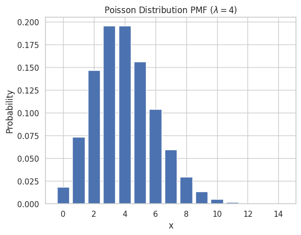
Plotting PMF for Poisson Distribution

To plot the PMF of a Poisson distribution, we can follow these steps:

1. Define a range of possible values for the Poisson distribution.
2. Compute the probabilities for each value using the PMF formula or a built-in function (e.g., poisson.pmf from scipy.stats).
3. Plot these probabilities using a bar chart.

x_poisson = np.arange(0, 15)
y_poisson = poisson.pmf(x_poisson, lambda_poisson)

sns.set(style="whitegrid")
plt.bar(x_poisson, y_poisson)
plt.title("Poisson Distribution PMF ($\lambda = 4$)")
plt.xlabel("x")
plt.ylabel("Probability")
plt.show()

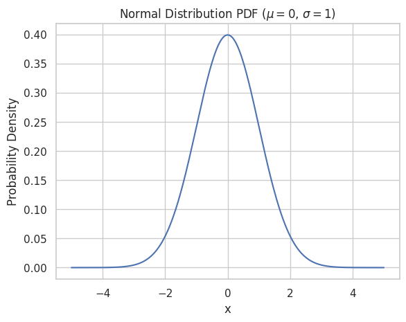
Plotting PDF for Normal Distribution

To plot the PDF of a normal distribution, we can follow these steps:

1. Create an array of evenly spaced points (e.g., using np.linspace) covering the desired range of the distribution.
2. Compute the probability density for each point using the PDF formula or a built-in function (e.g., norm.pdf from scipy.stats).
3. Plot these densities using a line chart.

x_normal = np.linspace(-5, 5, 1000)
y_normal = norm.pdf(x_normal, mu_normal, sigma)

sns.set(style="whitegrid")
plt.plot(x_normal, y_normal)
plt.title("Normal Distribution PDF ($\mu = 0$, $\sigma = 1$)")
plt.xlabel("x")
plt.ylabel("Probability Density")
plt.show()

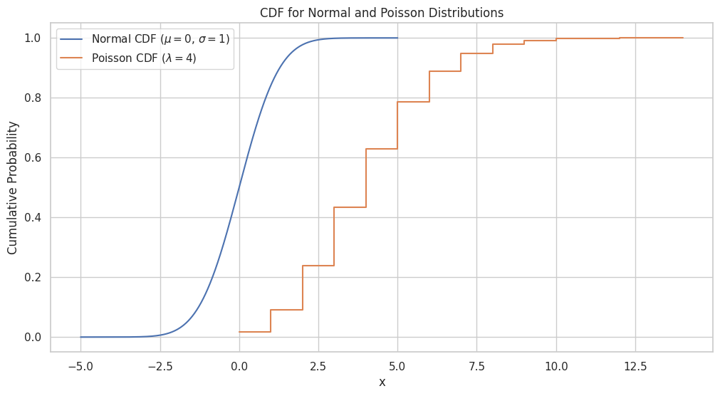
Plotting CDF for Normal and Poisson Distributions

To plot the CDF of the normal and Poisson distributions, we can follow these steps:

1. Create an array of evenly spaced points (e.g., using np.linspace) covering the desired range of the distribution.
2. Compute the cumulative probability for each point using the CDF formula or a built-in function (e.g., norm.cdf and poisson.cdf from scipy.stats).
3. Plot these cumulative probabilities using a line chart.

x_normal_cdf = np.linspace(-5, 5, 1000)
y_normal_cdf = norm.cdf(x_normal_cdf, mu_normal, sigma)

x_poisson_cdf = np.arange(0, 15)
y_poisson_cdf = poisson.cdf(x_poisson_cdf, lambda_poisson)

plt.figure(figsize=(12, 6))

sns.set(style="whitegrid")
plt.plot(x_normal_cdf, y_normal_cdf, label="Normal CDF ($\mu = 0$, $\sigma = 1$)")
plt.step(x_poisson_cdf,y_poisson_cdf, label="Poisson CDF ($\lambda = 4$)", where='post')
plt.title("CDF for Normal and Poisson Distributions")
plt.xlabel("x")
plt.ylabel("Cumulative Probability")
plt.legend(loc="upper left")
plt.show()