What is binomial distribution

A binomial distribution is a distribution that follows a probability p of an event occurring X times n observations of that event. Binomial distribution is sometimes denoted as B(n,p).

For example, the distribution of the number of times X that a 1 (p=\frac{1}{6}) occurs after three dice rolls (n = 3) follows a binomial distribution.

The probability of the binomial distribution is expressed by the following equation.

Dice Example

Let's consider the distribution of the number of times a dice rolls 1 three times.

First, let's consider the events. There are the following two patterns of events.

• 1 is rolled.
• 1 is not rolled.

Since there are two choices of occurrence or non-occurrence, the distribution of the probability of this event is a binomial distribution.

Next, let us consider the probability of the event occurring: the probability of the eye 1 occurring and the probability of the eye 1 not occurring are respectively as follows.

There are four patterns of how many times the dice will roll a 1 after three throws: 0, 1, 2, and 3 times. The probabilities of each are as follows.

A general description of the above probabilities is the following binomially distributed probability equation.

Checking with Python

Let's check the distribution of B(3,\frac{1}{6}) using Python. The code is as follows. The sample size is 1,000.

from scipy.stats import binom
import seaborn as sns
from matplotlib import pyplot as plt
%matplotlib inline

sns.set()
sns.set_context(rc = {'patch.linewidth': 0.2})
sns.set_style('dark')

data_binom = binom.rvs(n=3, p=1/6, size=1000)
plt.figure(figsize=(10,5))
sns.distplot(data_binom, kde=False)

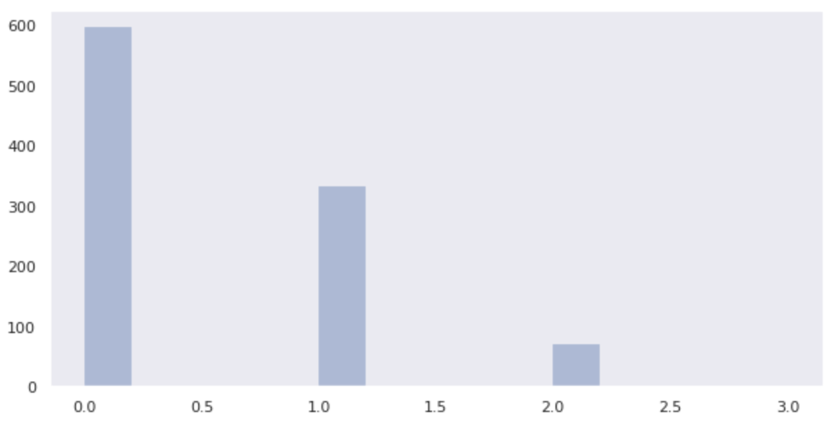
It can be seen that the probabilities are close to the calculated values of the following probabilities.

Laplace's Theorem

When a random variable X follows a binomial distribution B(n,p), it approaches a normal distribution as n is made sufficiently large. This is called Laplace's Theorem.

Let's check Laplace's theorem in Python. This time, we will check the distribution B(100,\frac{1}{6}) of the number of 1's obtained by throwing the dice 100 times. The sample size is 1,000.

from scipy.stats import binom
import seaborn as sns
from matplotlib import pyplot as plt
%matplotlib inline

sns.set()
sns.set_context(rc = {'patch.linewidth': 0.2})
sns.set_style('dark')

data_binom = binom.rvs(n=100, p=1/6, size=1000)
plt.figure(figsize=(10,5))
sns.distplot(data_binom, kde=False)

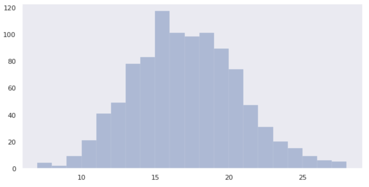
You can see that the distribution is closer to a normal distribution than when the dice are thrown three times.