What is beta distribution

Beta distribution is a probability distribution that the success rate $x$ of an event follows when the number of successes $\alpha$ and failures $\beta$ of a given trial are known. For example, if a coin toss is repeated 10 times and the front $\alpha$ comes up 7 times and the back $\beta$ comes up 3 times, then the success rate (probability of coming up with the front) follows the beta distribution.

The probability density function of the beta distribution is expressed by the following equation.

f(x) = {\frac{x^{\alpha -1}(1-x)^{\beta -1}}{B(\alpha ,\beta)}}

B(\alpha, \beta) = \int_{0}^{1}x^{\alpha-1}(1-x)^{\beta-1}dx

The beta distribution is flexible in shape depending on the values of $\alpha$ and $\beta$ , as the figure below shows.

Beta distribution

Therefore, it is frequently used in Bayesian statistics because it is easy to treat as a prior probability distribution.

Effect of α on beta distribution

Depending on the value of $\alpha$ in the beta distribution, the shape of the distribution is as follows.

Beta distribution alpha

Effect of β on beta distribution

The $\beta$ of the beta distribution has the following distribution shape depending on the value.

Beta distribution beta

Expected value and variance of beta distribution

The expected value and variance of the beta distribution are respectively:

E(X)=\frac{\alpha}{\alpha + \beta}

V(X)=\frac{\alpha \beta}{(\alpha + \beta)^2(\alpha + \beta + 1)}

Python Code

The Python code used in this article is as follows.

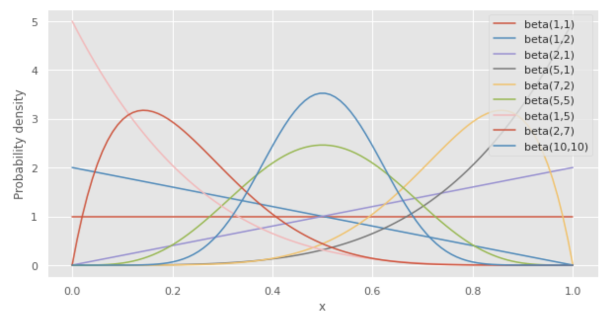
Draw beta distributions

import numpy as np
from scipy.stats import beta
import matplotlib.pyplot as plt

plt.style.use('ggplot')
fig, ax = plt.subplots(facecolor="w", figsize=(10, 5))

# x axis
x = np.linspace(0, 1, 100)

# draw graph
plt.plot(x, beta.pdf(x, 1, 1), label='beta(1,1)')
plt.plot(x, beta.pdf(x, 1, 2), label='beta(1,2)')
plt.plot(x, beta.pdf(x, 2, 1), label='beta(2,1)')
plt.plot(x, beta.pdf(x, 5, 1), label='beta(5,1)')
plt.plot(x, beta.pdf(x, 7, 2), label='beta(7,2)')
plt.plot(x, beta.pdf(x, 5, 5), label='beta(5,5)')
plt.plot(x, beta.pdf(x, 1, 5), label='beta(1,5)')
plt.plot(x, beta.pdf(x, 2, 7), label='beta(2,7)')
plt.plot(x, beta.pdf(x, 10, 10), label='beta(10,10)')
plt.legend()
plt.xlabel("x")
plt.ylabel("Probability density")
plt.show()

Beta distribution

Draw the impact of α

import numpy as np
from scipy.stats import beta
import matplotlib
import matplotlib.pyplot as plt
from matplotlib import animation, rc
from matplotlib.animation import FuncAnimation

rc('animation', html='html5')
np.random.seed(5)

# Set up formatting for the movie files
Writer = animation.writers['ffmpeg']
writer = Writer(fps=15, metadata=dict(artist='Me'), bitrate=1800)

prob_vals = np.arange(start=0.1, stop=10.01, step=0.2)

plt.style.use('ggplot')
fig = plt.figure(figsize=(10, 5))

# x axis
x = np.linspace(0, 1, 100)

def update(i):
    # initialize the graph of the previous frame
    plt.cla()
    p = prob_vals[i]

    # draw graph
    plt.plot(x, beta.pdf(x, round(p, 1), 2))
    plt.title(f'$alpha={str(round(p, 1))}, beta=2$', loc='left')
    plt.xlabel("x")
    plt.ylabel("Probability density")
    plt.ylim(0.1, 10.1)
    plt.xticks(ticks=[0, 1]) # x axis ticks

anime_prob = FuncAnimation(fig, update, frames=len(prob_vals), interval=1000)
anime_prob.save('beta_dist_alpha.gif', writer='pillow', fps=10)

Beta distribution alpha

Draw the impact of β

import numpy as np
from scipy.stats import beta
import matplotlib
import matplotlib.pyplot as plt
from matplotlib import animation, rc
from matplotlib.animation import FuncAnimation

rc('animation', html='html5')
np.random.seed(5)

# Set up formatting for the movie files
Writer = animation.writers['ffmpeg']
writer = Writer(fps=15, metadata=dict(artist='Me'), bitrate=1800)

prob_vals = np.arange(start=0.1, stop=10.01, step=0.2)

plt.style.use('ggplot')
fig = plt.figure(figsize=(10, 5))

# x axis
x = np.linspace(0, 1, 100)

def update(i):
    # initialize the graph of the previous frame
    plt.cla()
    p = prob_vals[i]

    # draw graph
    plt.plot(x, beta.pdf(x, 2, round(p, 1)))
    plt.title(f'$alpha=2, beta={str(round(p, 1))}$', loc='left')
    plt.xlabel("x")
    plt.ylabel("Probability density")
    plt.ylim(0.1, 10.1)
    plt.xticks(ticks=[0, 1]) # x axis ticks

anime_prob = FuncAnimation(fig, update, frames=len(prob_vals), interval=1000)
anime_prob.save('beta_dist_beta.gif', writer='pillow', fps=10)

Beta distribution beta

Beta distribution

What is beta distribution

Effect of α on beta distribution

Effect of β on beta distribution

Expected value and variance of beta distribution

Python Code

Draw beta distributions

Draw the impact of α

Draw the impact of β

Normal distribution

Gamma distribution

Ryusei Kakujo