What is the Normal Distribution

The normal distribution (Gaussian distribution) is one of the most universally utilized probability distributions and is used to describe natural and social phenomena. The normal distribution has the following basic properties:

• Mean, median, and mode are consistent.
• The curve is symmetrical with the mean value as the peak and the mean value as the center.
• The standard deviation changes the peak of the curve and the width of the distribution.
• The x-axis is an asymptote.
• The area bounded by the curve and the x-axis is 1

An example of a normal distribution is the height of an adult male (female).

Probability density function (PDF)

When a univariate random variable X follows a normal distribution with mean \mu and variance \sigma^2, its probability density function (RDF) is expressed by

A normal distribution is expressed as following N(\mu, \sigma^2) when it follows a mean \mu and variance \sigma^2. Also, the sum of the probability density function of the normal distribution is 1. In other words, integrating this probability density function over the entire interval yields 1.

How to derive the probability density function

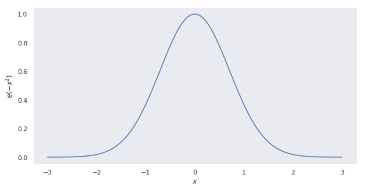
Most of the phenomena in the world have a peak at the mean value, and the probability of occurrence decreases as one moves away from the mean value. These phenomena can be expressed by the following function.

We will modify the above function into a more generic function based on the above. First, we will make it possible to set an arbitrary mean value. We can translate the mean value to the left or right depending on the value of \mu as follows.

Next, to allow the width of the distribution to be set arbitrarily, we transform the formula into the following:

The width of the distribution can now be controlled by the value of \sigma. Here, \sigma^2 in 2\sigma^2 is squared so that it always takes a positive value regardless of the value of \sigma. The coefficient of 2 is added to simplify the results of later integrations.

The density function is the sum of integrals over all intervals. Therefore, a constant c is added to the beginning of the equation to adjust it.

Computing the above equation, the constant c takes the following value:

Thus, the probability density function of the normal distribution is the following equation:

Probability of a normal distribution

For a normal distribution, if we know the mean \mu and standard deviation \sigma, we know the probability of occurrence of the random variable X.

The graph of the normal distribution below shows the range of standard deviations (± \sigma, ±1.96 \sigma, ±2 \sigma).

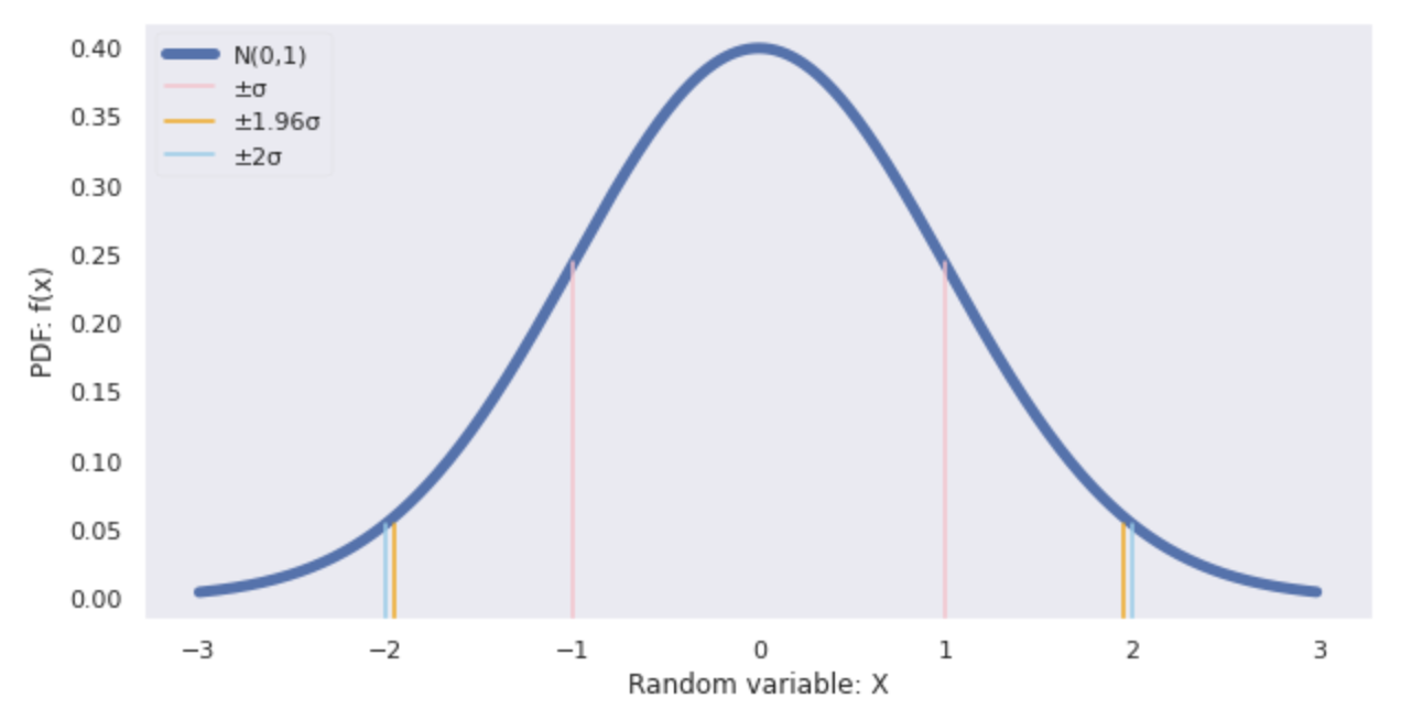
The range of the random variable X and its probability of occurrence are as follows.

The commonly used 1.96 \sigma in hypothesis-testing is treated as the 95% significance level.

Standard normal distribution

When the random variable X follows a normal distribution N(\mu,\sigma^2), aX+b follows a normal distribution N(a\mu+b,a^2\sigma^2).

Using this property and transforming Z=X-\mu\sigma, Z follows a normal distribution with mean 0 and variance 1. This transformation is called standardization of the normal distribution, and the normal distribution with mean 0 and variance 1 is called the standard normal distribution.

Reproductive property of the normal distribution

The reproductive property of normal distribution means that when random variables X and Y independently follow normal distributions N(\mu_1,\sigma^2_1) and N(\mu_2,\sigma^2_2) respectively, the distribution of X+Y is normal distribution The property that N(\mu_1+\mu_2,\sigma^2_1+\sigma^2_2).

As an example, assume that the mutually independent random variables X and Y follow N(2, 2^2) and N(5, 3^2), respectively, and find the probability distribution that the random variable 3X + 2Y follows.

The probability distribution that the random variable 3X follows is as follows:

The probability distribution that the random variable 2Y follows is as follows:

From the reproductive property of the normal distribution, the probability distribution that the random variable 3X + 2Y follows is

The probability distribution that the random variable 3X + 2Y follows is a normal distribution with expected value 16 and variance 72.

Python code

The Python code used in this article is as follows.

Draw y=e^{-x^2}

```python
import matplotlib.pyplot as plt
import seaborn as sns
import numpy as np
from matplotlib import rcParams
rcParams['figure.figsize'] = 10, 5
# %matplotlib inline

sns.set()
sns.set_context(rc = {'patch.linewidth': 0.2})
sns.set_style('dark')

x = np.linspace(-3, 3, 100)
y = np.exp(x)

plt.figure()
plt.plot(x, np.exp(-x**2))
plt.xlabel('$x$')
plt.ylabel('$-\exp(-x^2)$')

plt.show()

Draw normal distribution

from scipy import stats
import matplotlib.pyplot as plt
import seaborn as sns
import numpy as np
from matplotlib import rcParams
rcParams['figure.figsize'] = 10, 5
# %matplotlib inline

sns.set()
sns.set_context(rc = {'patch.linewidth': 0.2})
sns.set_style('dark')

# normal distribution setting
mean = 0
std  = 1

# set random variable
X = np.arange(-3,3,0.01)

# calculate PDF
Y = stats.norm.pdf(X,mean,std)

# draw normal distribution
plt.plot(X,Y,label="N(0,1)", linewidth=5)

# draw standard deviation
plt.axvline(x=std, color="pink", ymax=1.5*Y.max(), label="±σ")
plt.axvline(x=-std, color="pink", ymax=1.5*Y.max())
plt.axvline(x=1.96*std, color="orange", ymax=0.4*Y.max(), label="±1.96σ")
plt.axvline(x=-1.96*std, color="orange", ymax=0.4*Y.max())
plt.axvline(x=2*std, color="skyblue", ymax=0.4*Y.max(), label="±2σ")
plt.axvline(x=-2*std, color="skyblue", ymax=0.4*Y.max())

# graph setting
plt.xlabel("Random variable: X")
plt.ylabel("PDF: f(x)")
plt.legend(loc="upper left")
plt.show()