


回帰分析とは
回帰分析とは、ある結果に対してどの因子がどれくらい影響を与えているかという因果関係を関数として表現する統計手法です。このとき、結果となる数値を目的変数、因子となる数値を説明変数といいます。
また、説明変数が1つの場合を単回帰分析、複数の場合を重回帰分析といいます。
回帰分析は、事象の予測や要因分析などで用いられ、ビジネス、アカデミア問わず広く使用されている統計手法になります。
回帰分析の例
以下に回帰分析の例を紹介します。
-
不動産の価格の予測
- 単回帰分析
- 目的変数:不動産価格
- 説明変数:敷地面積
- 重回帰分析
- 目的変数:不動産価格
- 説明変数:敷地面積、駅との距離、築年数など
- 単回帰分析
-
広告のクリック率の予測
- 単回帰分析
- 目的変数:クリック率
- 説明変数:タイトル
- 重回帰分析
- 目的変数:クリック率
- 説明変数:タイトル、フォント、ジャンルなど
- 単回帰分析
Python で回帰分析
Pythonでの回帰分析の実装コードを紹介します。今回はデータセットとしてsklearnのボストン住宅価格データを利用します。
import pandas as pd
from sklearn import datasets

boston = datasets.load_boston()
df = pd.DataFrame(boston.data, columns=boston.feature_names)
df["PRICE"] = boston.target
df.head()
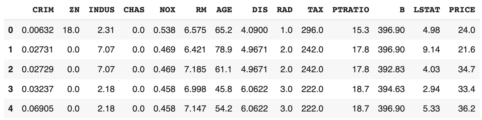
PRICEラベルが住宅価格で、残りのラベルが住宅の特徴のデータになっています。
各列のラベルの詳細はDESCRにより確認することができます。
print(boston.DESCR)
.. _boston_dataset:

Boston house prices dataset
---------------------------

**Data Set Characteristics:**

    :Number of Instances: 506

    :Number of Attributes: 13 numeric/categorical predictive. Median Value (attribute 14) is usually the target.

    :Attribute Information (in order):
        - CRIM     per capita crime rate by town
        - ZN       proportion of residential land zoned for lots over 25,000 sq.ft.
        - INDUS    proportion of non-retail business acres per town
        - CHAS     Charles River dummy variable (= 1 if tract bounds river; 0 otherwise)
        - NOX      nitric oxides concentration (parts per 10 million)
        - RM       average number of rooms per dwelling
        - AGE      proportion of owner-occupied units built prior to 1940
        - DIS      weighted distances to five Boston employment centres
        - RAD      index of accessibility to radial highways
        - TAX      full-value property-tax rate per $10,000
        - PTRATIO  pupil-teacher ratio by town
        - B        1000(Bk - 0.63)^2 where Bk is the proportion of black people by town
        - LSTAT    % lower status of the population
        - MEDV     Median value of owner-occupied homes in $1000's

    :Missing Attribute Values: None

    :Creator: Harrison, D. and Rubinfeld, D.L.

This is a copy of UCI ML housing dataset.
https://archive.ics.uci.edu/ml/machine-learning-databases/housing/


This dataset was taken from the StatLib library which is maintained at Carnegie Mellon University.

The Boston house-price data of Harrison, D. and Rubinfeld, D.L. 'Hedonic
prices and the demand for clean air', J. Environ. Economics & Management,
vol.5, 81-102, 1978.   Used in Belsley, Kuh & Welsch, 'Regression diagnostics
...', Wiley, 1980.   N.B. Various transformations are used in the table on
pages 244-261 of the latter.

The Boston house-price data has been used in many machine learning papers that address regression
problems.

.. topic:: References

   - Belsley, Kuh & Welsch, 'Regression diagnostics: Identifying Influential Data and Sources of Collinearity', Wiley, 1980. 244-261.
   - Quinlan,R. (1993). Combining Instance-Based and Model-Based Learning. In Proceedings on the Tenth International Conference of Machine Learning, 236-243, University of Massachusetts, Amherst. Morgan Kaufmann.
データセットを訓練データとテストデータに分割します。
from sklearn.model_selection import train_test_split

x_train, x_test, y_train, y_test = train_test_split(
  boston.data,
  boston.target,
  random_state=0
)
単回帰分析
単回帰分析では、1つの説明変数で目的変数を予測します。
pythonのsklearnを使って、RMというラベルを説明変数とします。
from sklearn import linear_model

x_rm_train = x_train[:, [5]]
x_rm_test = x_test[:, [5]]

model = linear_model.LinearRegression()
model.fit(x_train_rm, y_train)
a = model.coef_
b = model.intercept_
print("a: ", a)
print("b: ", b)
a:  [9.31294923]
b:  -36.180992646339206
データとモデルを可視化してみます。
import matplotlib.pyplot as plt

plt.scatter(x_rm_train, y_train, label="Train")
plt.scatter(x_rm_test, y_test, label="Test")

y_pred = model.predict(x_rm_train)
plt.plot(x_rm_train, y_pred, c="black")

plt.xlabel("RM")
plt.ylabel("PRICE")
plt.legend()
plt.show()
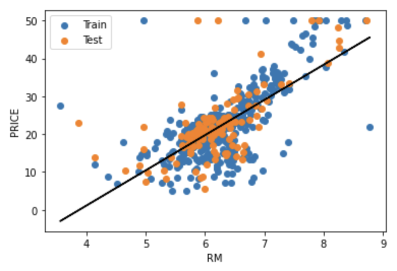
Trainが訓練データ、Testがテストデータ、黒の直線がモデルになっています。
決定係数
モデルの決定係数
ここで、
r2_scoreという関数で簡単に計算することができます。次のコードは訓練データとテストデータのそれぞれで
from sklearn.metrics import r2_score

y_pred_train = model.predict(x_rm_train)
print("R2 (train): ", r2_score(y_train, y_pred_train))

y_pred_test = model.predict(x_rm_test)
print("R2 (test): ", r2_score(y_test, y_pred_test))
R2 (train): 0.48752067939343646
R2 (test): 0.4679000543136781
MSE
モデルの MSE(Mean Squared Error) を計算します。MSEは
MSEが小さいほどモデルの誤差が小さいと解釈することができます。
次のコードは訓練データとテストデータそれぞれでMSEを計算します。
from sklearn.metrics import mean_squared_error

print("MSE (train): ", mean_squared_error(y_train, y_pred_train))

print("MSE (test): ", mean_squared_error(y_test, y_pred_test))
MSE (train):  43.71870658739849
MSE (test):  43.472041677202206
重回帰分析
重回帰分析では、複数の説明変数で目的変数を予測します。重回帰モデルは、
今回は全ての説明変数を使って重回帰分析を行います。
model = linear_model.LinearRegression()

model.fit(x_train, t_train)

a_df = pd.DataFrame(boston.feature_names, columns=["Exp"])
a_df["a"] = pd.Series(model.coef_)
a_df
| Exp | a | |
|---|---|---|
| 0 | CRIM | -0.117735 |
| 1 | ZN | 0.044017 |
| 2 | INDUS | -0.005768 |
| 3 | CHAS | 2.393416 |
| 4 | NOX | -15.589421 |
| 5 | RM | 3.768968 |
| 6 | AGE | -0.007035 |
| 7 | DIS | -1.434956 |
| 8 | RAD | 0.240081 |
| 9 | TAX | -0.011297 |
| 10 | PTRATIO | -0.985547 |
| 11 | B | 0.008444 |
| 12 | LSTAT | -0.499117 |
print("b: ", model.intercept_)
b: 36.93325545712031
決定係数
訓練データとテストデータのそれぞれで決定係数を計算します。
from sklearn.metrics import r2_score

y_pred_train = model.predict(x_rm_train)
print("R2 (train): ", r2_score(y_train, y_pred_train))

y_pred_test = model.predict(x_rm_test)
print("R2 (test): ", r2_score(y_test, y_pred_test))
R2 (train): 0.7697699488741149
R2 (test): 0.635463843320211
単回帰モデルと比較して
MSE
訓練データとテストデータのそれぞれでMSEを計算します。
from sklearn.metrics import mean_squared_error

print("MSE (train): ", mean_squared_error(y_train, y_pred_train))

print("MSE (test): ", mean_squared_error(y_test, y_pred_test))
MSE (train):  19.640519427908046
MSE (test):  29.78224509230252
単回帰モデルと比較してMSEが小さくなりました。しかし、テストデータのMSEは訓練データのMSEよりも大幅に大きくなりました。つまり、モデルが訓練データに過剰に適合してしまっている可能性があります。このように、モデルの良し悪しは
参考
/ja/articles/loss-functon


Ryusei Kakujo


Weave the future of cities through data
Transportation modeling/ Urban planning/ Machine learning/ Computer science/ GIS