What is a statistical model

A statistical model is a mathematical model that explains patterns or laws about observed data. It selects a probability distribution according to the characteristics of the data and estimates the parameters of the probability distribution that can successfully explain the observed data.

Parameter estimation

I will perform parameter estimation in Python for the following sample data with a sample size of 50.

data = [2,2,4,6,4,5,2,3,1,2,0,4,3,3,3,3,4,2,7,2,4,3,3,3,4,
        3,7,5,3,1,7,6,4,6,5,2,4,7,2,2,6,2,4,5,4,5,1,3,2,3]

Data investigation

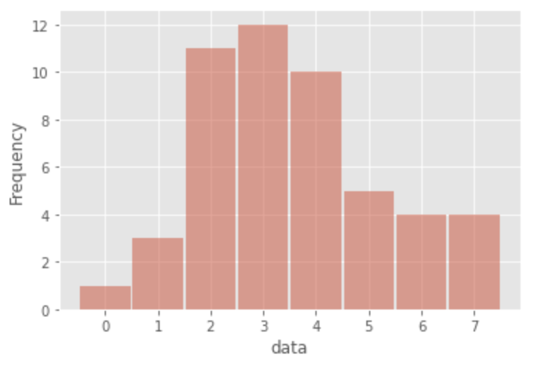
First, let us look at a histogram of the data.

import matplotlib.pyplot as plt
import seaborn as sns
%matplotlib inline

plt.style.use('ggplot')
plt.figure(figsize=(10,5))

data = [2,2,4,6,4,5,2,3,1,2,0,4,3,3,3,3,4,2,7,2,4,3,3,3,4,
        3,7,5,3,1,7,6,4,6,5,2,4,7,2,2,6,2,4,5,4,5,1,3,2,3]

plt.hist(data, bins = [-0.5 + v for v in range(max(data) + 2)], alpha=0.5, rwidth=0.95)
plt.xlabel('data')
plt.ylabel('Frequency')

Next let us look at a summary of the data.

import pandas as pd

df = pd.DataFrame(data, columns=['x'])
df.describe()

Let us look at the sample variance.

# sample variabce
df.var()

2.986122

The survey confirmed the following:

• Mountain-like distribution
• Data are count data (non-negative integers)
• Sample mean is 3.56
• Sample variance is 2.99

Assumptions of probability distribution

From the sample data, we assume a probability distribution that the population follows. We know the following about the sample data.

• The data is count data
• The lower bound is 0 but the upper bound is unknown
• The sample mean is 3.56 and the sample variance is 2.99, which are relatively close

From the above characteristics, we assume a Poisson distribution with \lambda=3.56.

Poisson distribution vs. sample distribution

Visualize the Poisson distribution of \lambda=3.56 and the sample data distribution superimposed.

fig, ax1 = plt.subplots()
plt.hist(data, bins = [-0.5 + v for v in range(max(data) + 2)], alpha=0.5, rwidth=0.95)
poisson_values = poisson.rvs(3.56, size=10000)
prod = (pd.value_counts(poisson_values) / 10000).sort_index()
ax2 = ax1.twinx()
ax2.plot(prod)
plt.show()

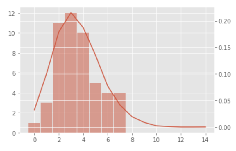
It appears that the distribution of the sample data can be represented by a Poisson distribution with \lambda=3.56.

Parameter estimation of the assumed probability distribution

The parameters of the probability distribution are estimated based on the sample data. Here we use a parameter estimation method called maximum likelihood estimation.

Maximum likelihood estimation is a parameter estimation method that searches for the parameter that maximizes the likelihood, a statistic that expresses how well it fits the observed data. In this case, the parameter is \lambda. In other words, we are estimating the value of \lambda that maximizes the fit to the data.

The likelihood is the product of the probabilities for all the sample data. The likelihood is a function of the parameter, denoted by L. Since the parameter in this case is \lambda, the expression for the likelihood is as follows

where y_i is the observed value. In this example, y_1=2, y_2=2, y_3=4, \cdots, y_{50}=3.

We examine \lambda that maximizes the likelihood L(\lambda). However, since the likelihood as it is is multiplicative and difficult to handle, the log-transformed log-likelihood is used for the maximum likelihood estimation of the parameters.

The following figure shows the shape of the distribution and the value of log L(\lambda) when the parameter \lambda is varied from 3.2 to 4.4.

import matplotlib.pyplot as plt
import pandas as pd
import seaborn as sns
import sympy
from scipy.stats import poisson
%matplotlib inline

plt.style.use('ggplot')
plt.figure(figsize=(10,5))

lams = np.arange(3.2,4.5,0.4)

for i, lam in enumerate(lams):
    log_l = 0
    for y in data:
        f = (lam**y)*sympy.exp(-lam)/sympy.factorial(y)
        logf=sympy.log(f)
        log_l = log_l + logf

    fig, ax = plt.subplots()
    ax.hist(data, bins = [-0.5 + v for v in range(max(data) + 2)], alpha=0.5, rwidth=0.95)
    poisson_values = poisson.rvs(lam, size=10000)
    prod = (pd.value_counts(poisson_values) / 10000).sort_index()
    ax2 = ax.twinx()
    ax2.plot(prod, label=f'lambda={round(lam, 1)}, log L={round(log_l, 1)}')
    plt.legend()
    plt.show()

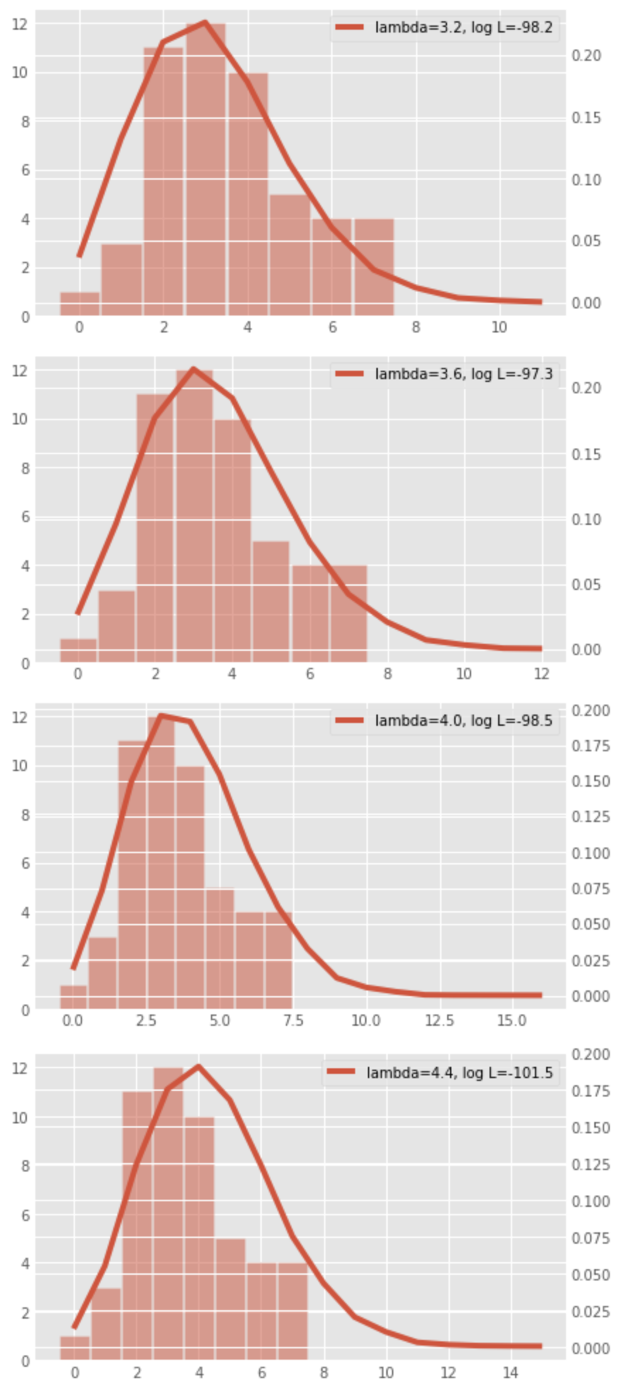
We can see that the log-likelihood is likely to be maximized around \lambda=3.6. Since log L is a monotonically increasing function of the likelihood L, the log likelihood is also maximum at \lambda where the log likelihood is maximum.

To derive the maximum log likelihood, we can find \lambda where the partial derivative of the log likelihood with parameter \lambda is 0.

Computing the above equation, we see that the likelihood is maximized when \lambda=3.56.

Which probability distribution should be used for statistical models

When choosing a probability distribution for a statistical model to explain observed data, following points need to be checked:

• Type of data (discrete or continuous)
• Range of data
• Relationship between sample variance and sample mean

For some probability distributions, the necessary conditions that may be used as probability distributions for statistical models are as follows.