2022-12-23

Generalized linear model

What is a Generalized Linear Model (GLM)?

Generalized Linear Model (GLM) is a statistical model that can be applied even when the objective variable follows a probability distribution other than the normal distribution.

Simple or multiple regression analysis is called a linear model and is a statistical model that assumes that the objective variable follows a normal distribution. If the objective variable cannot be assumed to follow a normal distribution, for example, if the objective variable is a discrete variable such as categorical or count data, the linear model is not applicable. GLM can handle not only the normal distribution but also other distributions called exponential distribution families such as binomial, gamma, and Poisson distributions.

In the GLM, the relationship between the objective and explanatory variables need not be a simple linear equation, but can be expressed as follows:

g(y) = \beta_0x_0 + \beta_1x_1 + \cdots + \beta_nx_n

$\beta$ is the parameter, $x$ is the explanatory variable, and $n$ is the number of explanatory variables. The right-hand side of the above equation is linearly coupled and is called the linear predictor. And, the left-hand side function $g(y)$ is called a link function.

Combination of probability distribution and link function

Commonly used combinations of probability distributions and link functions are as below table.

	Probability distribution	Link function
Discrete	Binomial distribution	logit
Discrete	Poisson distribution	log
Discrete	Negative binomial distribution	log
Continuous	Gamma distribution	log
Continuous	Normal distribution	identity

Constructing the GLM

Let us actually construct the GLM. Let us consider the seed count data of 100 fictitious plants. The data consists of the following columns:

y: Number of seeds of the individuals
x: Size of individuals
f: whether the individuals have been treated with fertilizer or not (C: without fertilizer, T: with fertilizer)

import pandas as pd

# number of seeds
y = [6,6,6,12,10,4,9,9,9,11,6,10,6,10,11,8,3,8,5,5,4,11,5,10,6,6,7,9,3,10,2,9,10,
     5,11,10,4,8,9,12,8,9,8,6,6,10,10,9,12,6,14,6,7,9,6,7,9,13,9,13,7,8,10,7,12,
     6,15,3,4,6,10,8,8,7,5,6,8,9,9,6,7,10,6,11,11,11,5,6,4,5,6,5,8,5,9,8,6,8,7,9]

# body size
x = [8.31,9.44,9.5,9.07,10.16,8.32,10.61,10.06,9.93,10.43,10.36,10.15,10.92,8.85,
     9.42,11.11,8.02,11.93,8.55,7.19,9.83,10.79,8.89,10.09,11.63,10.21,9.45,10.44,
     9.44,10.48,9.43,10.32,10.33,8.5,9.41,8.96,9.67,10.26,10.36,11.8,10.94,10.25,
     8.74,10.46,9.37,9.74,8.95,8.74,11.32,9.25,10.14,9.05,9.89,8.76,12.04,9.91,
     9.84,11.87,10.16,9.34,10.17,10.99,9.19,10.67,10.96,10.55,9.69,10.91,9.6,
     12.37,10.54,11.3,12.4,10.18,9.53,10.24,11.76,9.52,10.4,9.96,10.3,11.54,9.42,
     11.28,9.73,10.78,10.21,10.51,10.73,8.85,11.2,9.86,11.54,10.03,11.88,9.15,8.52,
     10.24,10.86,9.97]

# feed (C: control, T: treatment)
f = ['C','C','C','C','C','C','C','C','C','C','C','C','C','C','C','C','C','C','C',
     'C','C','C','C','C','C','C','C','C','C','C','C','C','C','C','C','C','C','C',
     'C','C','C','C','C','C','C','C','C','C','C','C','T','T','T','T','T','T','T',
     'T','T','T','T','T','T','T','T','T','T','T','T','T','T','T','T','T','T','T',
     'T','T','T','T','T','T','T','T','T','T','T','T','T','T','T','T','T','T','T',
     'T','T','T','T','T']

df = pd.DataFrame(list(zip(y, x, f)), columns =['y', 'x', 'f'])

display(df.head())

	y	x	f
0	6	8.31	C
1	6	9.44	C
2	6	9.50	C
3	12	9.07	C
4	10	10.16	C

Data investigation

Let us check descriptive statistics.

df.describe()

	y	x
count	100.000000	100.000000
mean	7.830000	10.089100
std	2.624881	1.008049
min	2.000000	7.190000
25%	6.000000	9.427500
50%	8.000000	10.155000
75%	10.000000	10.685000
max	15.000000	12.400000

Displays the number of C and T for f, respectively.

print('num of C:', len(df[df['f'] == 'C']))
print('num of T:', len(df[df['f'] == 'T']))

num of C: 50
num of T: 50

Descriptive statistics of the data confirm the following:

Number of seeds y:
- Non-negative integers (2 to 15).
- Mean and variance are fairly close.
Size of individuals x:
- Positive real numbers (continuous values)
- Variance is small.
Fertilizer treatment f:
- It is a categorical variable.
- The number of elements in each category is equal.

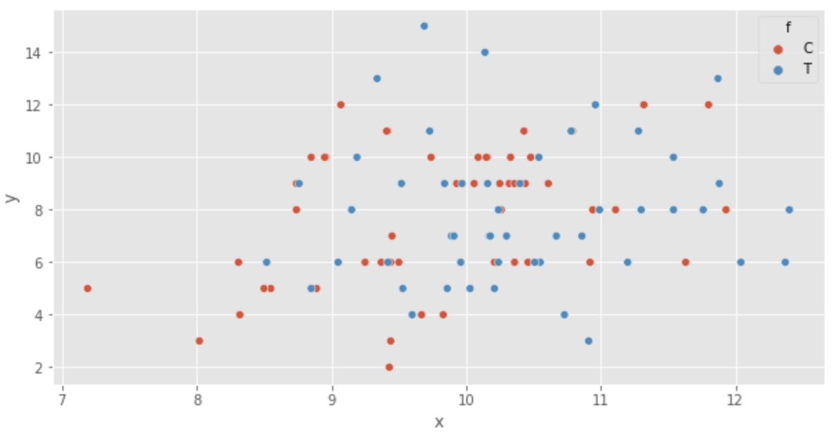
Next, we visualize the data. First, a scatter plot is displayed.

import matplotlib.pyplot as plt
import seaborn as sns
%matplotlib inline

plt.style.use('ggplot')
plt.figure(figsize=(10,5))
sns.set(rc={'figure.figsize':(10,5)})

sns.scatterplot(x='x', y='y', hue='f', data=df)

Scatter of f

Displays a box-and-whisker diagram.

sns.boxplot(x='f', y='y', data=df)

Box of f

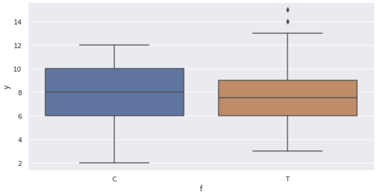
The graph confirms the following:

As size $x$ increases, the number of seeds y also increases (scatter plot)
There appears to be no effect of fertilizer (box-and-whisker diagram)

Building a statistical model with Poisson regression

Assume that the number of seeds $y_i$ of some fictitious plant individual $i$ follows a Poisson distribution. The probability distribution of the Poisson distribution is the following equation

P(X=y| \lambda) = \frac{e^{-\lambda} \lambda^y_i}{y_i!}

The Poisson distribution has a parameter $\lambda$ that determines the shape of the distribution, but $\lambda$ (mean number of seeds) is different for each individual, and we believe that the number of seeds is determined from a Poisson distribution with a different shape for each individual. In this article, let us construct statistical models for the following three patterns.

Statistical model where number of seeds depends on the size of the individual
Statistical model where number of seeds depends on the presence or absence of fertilizer treatment
Statistical model where number of seeds depends on the size of the individual and the presence or absence of fertilizer treatment.

Statistical model where number of seeds depends on the size of the individual

Let us first define $\lambda_i$ as a function of individual size $x_i$ as follows.

\lambda_i = e^{\beta_1 + \beta_2x_i}

where $\beta_1$ and $\beta_2$ are called parameters or coefficients and $\beta_1$ is called the intercept.

Taking the logarithm of both sides, we get

\log (\lambda_i) = \beta_1 + \beta_2 x_i

The right-hand side $\beta_1 + \beta_2 x_i$ is called the linear predictor because it is a linear combination.

The function on the left-hand side for the linear predictor is called the link function. This time the link function is $\log (\lambda_i)$ and is logarithmic, so it is called the log link function.

The log link function is often used in the GLM for Poisson regression. The reason is that the mean $\lambda$ of the Poisson distribution must be non-negative. This is convenient because $\lambda_i = e^{linear\_predictor} \geqq 0$ and it is non-negative.

From this we estimate $\beta_1$ and $\beta_2$ that maximize the following log-likelihood functions.

\log L(\beta_1, \beta_2) = \sum_i \log \frac{\lambda_i^{y_i}e^{-\lambda_i}}{y_i!}

Parameter estimation is easily accomplished with the following Python code.

import statsmodels.api as sm
import statsmodels.formula.api as smf

fit_x = smf.glm('y ~ x', data=df, family=sm.families.Poisson()).fit()
fit_x.summary()

Poisson regression | x

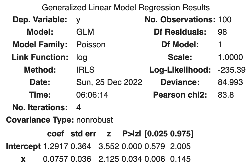
The following results were obtained.

	coef	std err	z	Log-likelihood
Intercept	1.2917	0.364	3.552
x	0.0757	0.036	2.125
				-235.39

std err is the standard error, i.e., the standard deviation of the estimated parameters. A normal distribution is assumed for the derivation of the standard deviation. z is the z-value.

The $\lambda$ (average number of seeds) is as follows.

\lambda_i = e^{1.2917 + 0.0757x_i}

Plot the above function.

import numpy as np
import math

sns.scatterplot(x='x', y='y', hue='f', data=df)
x = np.arange(df.x.min(), df.x.max() + 0.01, 0.01)
y = [math.exp(fit_x.params['Intercept'] + fit_x.params['x'] * x_i)  for x_i in x]
plt.plot(x, y)

Predict | x

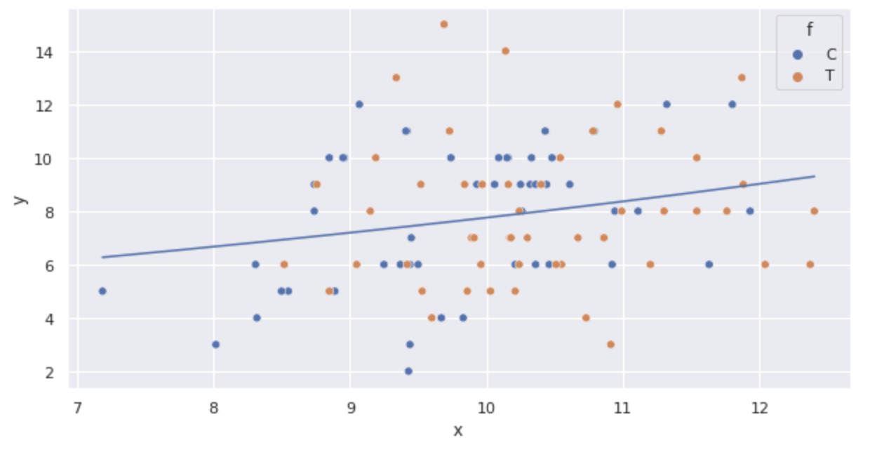
The line is drawn that the average seed count increases as size $x$ increases.

Statistical model where number of seeds depends on the presence or absence of fertilizer treatment

Let us consider a model that incorporates fertilizer application status $f_i$ as an explanatory variable.

Fertilizer application $f_i$ is a categorical variable. Categorical variables are usually replaced by dummy variables. Fertilizer application $f_i$ is replaced by a dummy variable $d_i$ as follows:

d_i = \left\{ \begin{array}{ll} 0 & (f_i = \mathrm{C}) \\ 1 & (f_i = \mathrm{T}) \end{array} \right.

The model is as follows.

\lambda_i = e^{\beta_1 + \beta_3 d_i}

That is, if individual $i$ has no fertilizer treatment ( $f_i=C$ ), then

\lambda_i = e^{\beta_i}

and if individual $i$ has a fertilizer treatment ( $f_i=T$ ), then

\lambda_i = e^{\beta_i + \beta_3}

Let us estimate $\beta_1$ and $\beta_2$ that maximize the following log-likelihood functions.

\log L(\beta_1, \beta_2) = \sum_i \log \frac{\lambda_i^{y_i}e^{-\lambda_i}}{y_i!}

import statsmodels.api as sm
import statsmodels.formula.api as smf

fit_f = smf.glm('y ~ f', data=df, family=sm.families.Poisson()).fit()
fit_f.summary()

Poisson regression | f

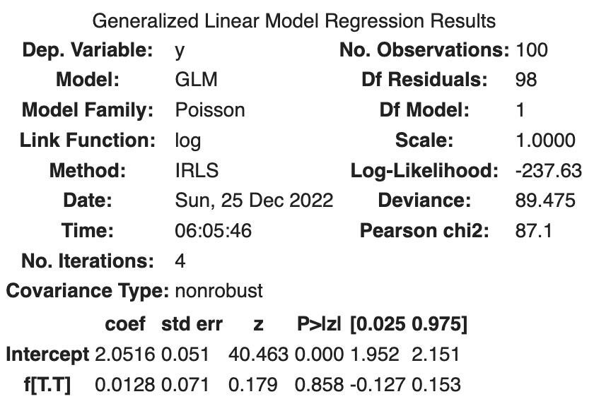
The following results were obtained.

	coef	std err	z	Log-likelihood
Intercept	2.0516	0.051	40.463
f[T.T]	0.0128	0.071	0.179
				-237.63

That is, $\lambda$ (average number of seeds) is as follows.

\lambda_i = e^{2.0516} \quad (f_i = \mathrm{C})

\lambda_i = e^{2.0516 + 0.0128} \quad (f_i = \mathrm{T})

The addition of the fertilizer treatment resulted in a slight increase in the average number of seeds.

The log-likelihood is -237.63, which is smaller than the log-likelihood of the model with $x_i$ as explanatory variable of -235.39. In other words, the model fits the data poorly.

Statistical model where number of seeds depends on the size of the individual and the presence or absence of fertilizer treatment

Finally, we consider a model that incorporates size $x_i$ and fertilizer treatment $f_i$ as explanatory variables.

The model is as follows

\lambda_i = e^{\beta_1 + \beta_2x_i + \beta_3 d_i}

Estimate $\beta_1$ , $\beta_2$ , and $\beta_3$ that maximize the following log-likelihood functions.

\log L(\beta_1, \beta_2, \beta_3) = \sum_i \log \frac{\lambda_i^{y_i}e^{-\lambda_i}}{y_i!}

import statsmodels.api as sm
import statsmodels.formula.api as smf

fit_full = smf.glm('y ~ x + f', data=df, family=sm.families.Poisson()).fit()
fit_full.summary()

Poisson regression | f

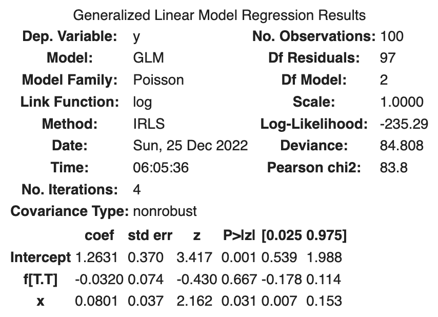
The following results were obtained.

	coef	std err	z	Log-likelihood
Intercept	1.2631	0.370	3.417
f[T.T]	-0.0320	0.074	-0.430
x	0.0801	0.037	2.162
				-235.29

The following results were obtained.

\lambda_i = e^{2.0516 + 0.0801 x_i} \quad (f_i = \mathrm{C})

\lambda_i = e^{2.0516 + 0.0801 x_i - 0.0320} \quad (f_i = \mathrm{T})

It is interpreted that the average seed count will be lower with fertilizer treatment. Specifically, $e^{-0.032} \approx 0.969$ indicates that the average number of seeds is 0.969 times higher after fertilizer application.

The log-likelihood is -235.29, which is a better fit to the data than the previous two models.