t 分布とは

t分布とは、標本平均 $\bar{X}$ を標本の標準偏差で標準化した値が従う確率分布です。

母集団の平均を $\mu$、標準偏差を $\sigma$ とすると，標本平均の分布は中心極限定理より、平均 $\mu$、分散 $\frac{\sigma^2}{n}$ の正規分布になります。標本平均を標準化した値であるz値は次のようになります。

上式zが従う分布である標準正規分布をもとに仮説検定が行われます。しかし、上式の母集団の標準偏差 $\sigma$ は通常未知の値です。そこで $\sigma$ の代わりとして標本の標準偏差 $s$ を使います。そのため、次の $t$ が従う分布を考えることになります。

$s^2$ は不偏分散とも言います。上式 $t$ が従う分布がt分布になります。つまり、t分布は標準正規分布を代替した分布と言えます。

t分布の確率密度関数は次の式で表されます。

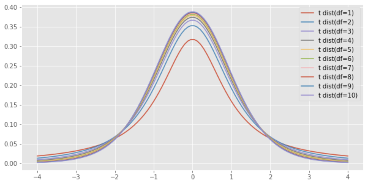
t分布の確率密度関数は自由度（$n$）のみで分布の形状が定まります。自由度が1から10のt分布のグラフは次のようになります。

自由度 $n$ が大きくなるにつれて標準正規分布に近づいていきます。

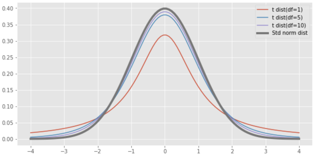
したがって、$n$ が十分に大きい場合は、母分散が未知の仮説検定において、標準正規分布の代用としてt分布を使うことができます。この検定をt検定と言います。

t 分布の期待値と分散

t分布の期待値、分散はそれぞれ以下になります。

t 分布表（上側）

t分布はパラメータが $n$ のみであるため、t分布の確率をt分布表と呼ばれる表にまとめることができます。以下に上側確率 $\alpha$ がそれぞれ，0.1，0.05，0.025，0.01，0.005に一致するt分布の自由度をまとめたt分布表を示します。

例えば、自由度20のt分布の上側5％点を求めたい場合は、$n=20$ と $\alpha=0.05$ の交差点の値を探します。したがって、求める上側5％点は1.725になります。

Python コード

以下にt分布の描画で使用したPythonコードを示します。

import numpy as np
from scipy import stats
import matplotlib.pyplot as plt

plt.style.use('ggplot')
fig, ax = plt.subplots(facecolor="w", figsize=(10, 5))

x = np.linspace(-4, 4, 100)
z = stats.norm.pdf(x, loc=0, scale=1)

for df in range(1, 11):
    t = stats.t.pdf(x, df)
    plt.plot(x, t, label=f"t dist(df={df})")
plt.legend()

import numpy as np
from scipy import stats
import matplotlib.pyplot as plt

plt.style.use('ggplot')
fig, ax = plt.subplots(facecolor="w", figsize=(10, 5))

x = np.linspace(-4, 4, 100)
z = stats.norm.pdf(x, loc=0, scale=1)

for df in [1, 5, 10]:
    t = stats.t.pdf(x, df)
    plt.plot(x, t, label=f"t dist(df={df})")
plt.plot(x, z, label='Std norm dist', linewidth=4)
plt.legend()