2023-02-17

言語処理100本ノック第7章：単語ベクトル

Machine Learning

NLP

はじめに

言語処理100本ノックというNLPに関する問題集が東京工業大学によって作成、管理されています。

https://nlp100.github.io/ja/ch07.html

この記事では、「第7章: 単語ベクトル」について回答例を紹介します。

60. 単語ベクトルの読み込みと表示

Google News データセット（約 1,000 億単語）での学習済み単語ベクトル（300 万単語・フレーズ，300 次元）をダウンロードし，”United States”の単語ベクトルを表示せよ．ただし，”United States”は内部的には”United_States”と表現されていることに注意せよ．

from gensim.models import KeyedVectors

model = KeyedVectors.load_word2vec_format('./GoogleNews-vectors-negative300.bin.gz', binary=True)
print(model['United_States'])

[-3.61328125e-02 -4.83398438e-02  2.35351562e-01  1.74804688e-01
 -1.46484375e-01 -7.42187500e-02 -1.01562500e-01 -7.71484375e-02
 .
 .
 .
 -8.49609375e-02  1.57470703e-02  7.03125000e-02  1.62353516e-02
 -2.27050781e-02  3.51562500e-02  2.47070312e-01 -2.67333984e-02]

61. 単語の類似度

“United States”と”U.S.”のコサイン類似度を計算せよ．

model.similarity('United_States', 'U.S.')

0.73107743

62. 類似度の高い単語 10 件

“United States”とコサイン類似度が高い 10 語と，その類似度を出力せよ．

model.most_similar('United_States', topn=10)

[('Unites_States', 0.7877248525619507),
 ('Untied_States', 0.7541370391845703),
 ('United_Sates', 0.74007248878479),
 ('U.S.', 0.7310774326324463),
 ('theUnited_States', 0.6404393911361694),
 ('America', 0.6178410053253174),
 ('UnitedStates', 0.6167312264442444),
 ('Europe', 0.6132988929748535),
 ('countries', 0.6044804453849792),
 ('Canada', 0.6019070148468018)]

63. 加法構成性によるアナロジー

“Spain”の単語ベクトルから”Madrid”のベクトルを引き，”Athens”のベクトルを足したベクトルを計算し，そのベクトルと類似度の高い 10 語とその類似度を出力せよ．

model.most_similar(
  positive=['Spain', 'Athens'],
  negative=['Madrid'],
  topn=10
)

[('Greece', 0.6898480653762817),
 ('Aristeidis_Grigoriadis', 0.560684859752655),
 ('Ioannis_Drymonakos', 0.5552908778190613),
 ('Greeks', 0.545068621635437),
 ('Ioannis_Christou', 0.5400862097740173),
 ('Hrysopiyi_Devetzi', 0.5248445272445679),
 ('Heraklio', 0.5207759737968445),
 ('Athens_Greece', 0.516880989074707),
 ('Lithuania', 0.5166865587234497),
 ('Iraklion', 0.5146791338920593)]

64. アナロジーデータでの実験

単語アナロジーの評価データをダウンロードし，vec(2 列目の単語) - vec(1 列目の単語) + vec(3 列目の単語)を計算し，そのベクトルと類似度がもっとも高い単語と，その類似度を求めよ．求めた単語と類似度は，各事例の末尾に追記せよ．

!wget http://download.tensorflow.org/data/questions-words.txt
!head -5 questions-words.txt

>> : capital-common-countries
>> Athens Greece Baghdad Iraq
>> Athens Greece Bangkok Thailand
>> Athens Greece Beijing China
>> Athens Greece Berlin Germany

with open('./questions-words.txt', 'r') as f1, open('./questions-words-add.txt', 'w') as f2:
  for line in f1:
    line = line.split()
    if line[0] == ':':
      category = line[1]
    else:
      word, cos = model.most_similar(positive=[line[1], line[2]], negative=[line[0]], topn=1)[0]
      f2.write(' '.join([category] + line + [word, str(cos) + '\n']))

!head -5 questions-words-add.txt

>> capital-common-countries Athens Greece Baghdad Iraq Iraqi 0.6351870894432068
>> capital-common-countries Athens Greece Bangkok Thailand Thailand 0.7137669324874878
>> capital-common-countries Athens Greece Beijing China China 0.7235777974128723
>> capital-common-countries Athens Greece Berlin Germany Germany 0.6734622120857239
>> capital-common-countries Athens Greece Bern Switzerland Switzerland 0.4919748306274414

65. アナロジータスクでの正解率

64 の実行結果を用い，意味的アナロジー（semantic analogy）と文法的アナロジー（syntactic analogy）の正解率を測定せよ．

with open('./questions-words-add.txt', 'r') as f:
  sem_cnt = 0
  sem_cor = 0
  syn_cnt = 0
  syn_cor = 0
  for line in f:
    line = line.split()
    if not line[0].startswith('gram'):
      sem_cnt += 1
      if line[4] == line[5]:
        sem_cor += 1
    else:
      syn_cnt += 1
      if line[4] == line[5]:
        syn_cor += 1

print(f'semantic analogy accuracy: {sem_cor / sem_cnt:.3f}')
print(f'syntactic analogy accuracy: {syn_cor / syn_cnt:.3f}')

>> semantic analogy accuracy: 0.731
>> syntactic analogy accuracy: 0.740

66. WordSimilarity-353 での評価

The WordSimilarity-353 Test Collection の評価データをダウンロードし，単語ベクトルにより計算される類似度のランキングと，人間の類似度判定のランキングの間のスピアマン相関係数を計算せよ．

!wget http://www.gabrilovich.com/resources/data/wordsim353/wordsim353.zip
!unzip wordsim353.zip
!head -5 './combined.csv'

>> Word 1,Word 2,Human (mean)
>> love,sex,6.77
>> tiger,cat,7.35
>> tiger,tiger,10.00
>> book,paper,7.46

import pandas as pd
import numpy as np
from scipy.stats import spearmanr

df = pd.read_csv('combined.csv')
df['sim'] = df.apply(lambda x: model.similarity(x['Word 1'], x['Word 2']), axis=1)
print(df.head(5))

correlation, pvalue = spearmanr(df['Human (mean)'], df['sim'])

print(f'\nspearman’s rank correlation : {correlation:.3f}')
print(f'pvalue : {pvalue}')

>>      Word 1    Word 2  Human (mean)       sim
>> 0      love       sex          6.77  0.263938
>> 1     tiger       cat          7.35  0.517296
>> 2     tiger     tiger         10.00  1.000000
>> 3      book     paper          7.46  0.363463
>> 4  computer  keyboard          7.62  0.396392
>>
>> spearman’s rank correlation : 0.700
>> pvalue : 2.86866666051422e-53

67. k-means クラスタリング

国名に関する単語ベクトルを抽出し，k-means クラスタリングをクラスタ数 k=5 として実行せよ．

from sklearn.cluster import KMeans

# get countries
countries = set()
with open('./questions-words-add.txt') as f:
  for line in f:
    line = line.split()
    if line[0] in ['capital-common-countries', 'capital-world']:
      countries.add(line[2])
    elif line[0] in ['currency', 'gram6-nationality-adjective']:
      countries.add(line[1])

# get country vectors
countries_vec = [model[country] for country in list(countries)]

# k-means clustering
kmeans = KMeans(n_clusters=5, random_state=42)
kmeans.fit(countries_vec)
for i in range(5):
  cluster = np.where(kmeans.labels_ == i)[0]
  print(f'cluster: {i}')
  print(', '.join([list(countries)[k] for k in cluster]))

cluster: 0
Rwanda, Uganda, Liberia, Burundi, Sudan, Somalia, Eritrea
cluster: 1
Australia, England, Sweden, Switzerland, Belgium, Denmark, Italy, Algeria, Portugal, France, Canada, Finland, Spain, Ireland, Norway, Germany
cluster: 2
Vietnam, Egypt, Lebanon, Iran, China, Qatar, Japan, Nepal, Pakistan, Iraq, Philippines, Thailand, Jordan, Indonesia, Bangladesh, Syria, Afghanistan, Bahrain
cluster: 3
Belarus, Slovenia, Ukraine, Kazakhstan, Serbia, Greece, Azerbaijan, Russia, Kyrgyzstan, Romania, Turkmenistan, Turkey, Moldova, Slovakia, Tajikistan, Hungary
cluster: 4
Jamaica, Guyana, Botswana, Malawi, Ghana, Nicaragua, Zambia, Venezuela, Mali, Samoa, Tuvalu, Madagascar, Belize, Guinea, Zimbabwe, Angola, Gabon, Gambia, Mozambique, Senegal, Nigeria, Peru, Cuba

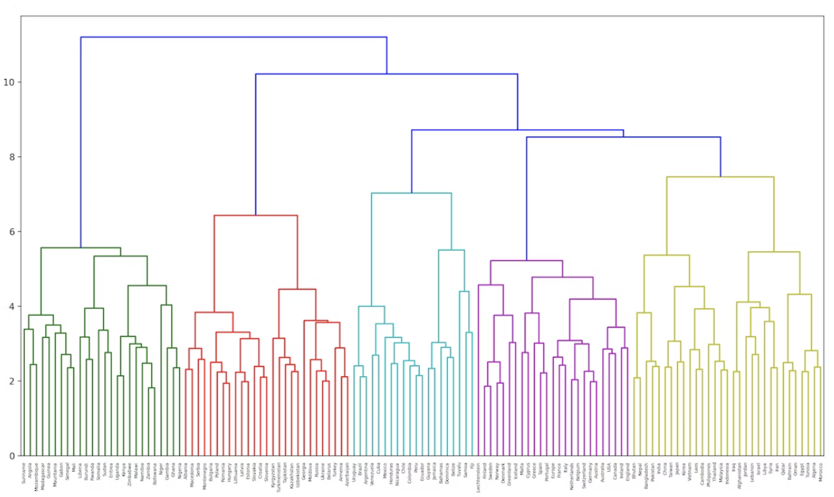
68. Ward 法によるクラスタリング

国名に関する単語ベクトルに対し，Ward 法による階層型クラスタリングを実行せよ．さらに，クラスタリング結果をデンドログラムとして可視化せよ．

from matplotlib import pyplot as plt
from scipy.cluster.hierarchy import dendrogram, linkage

plt.figure(figsize=(15,5))
Z = linkage(countries_vec, method='ward')
dendrogram(Z, labels=countries)
plt.show()

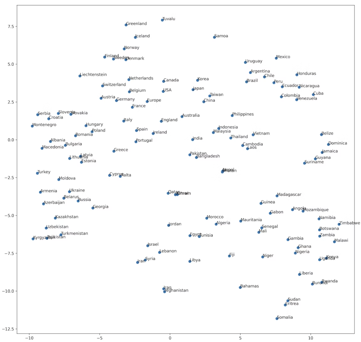
69. t-SNE による可視化

ベクトル空間上の国名に関する単語ベクトルを t-SNE で可視化せよ．

!pip install bhtsne

import bhtsne

embedded = bhtsne.tsne(np.array(countries_vec).astype(np.float64), dimensions=2, rand_seed=123)
plt.figure(figsize=(10, 10))
plt.scatter(np.array(embedded).T[0], np.array(embedded).T[1])
for (x, y), name in zip(embedded, countries):
    plt.annotate(name, (x, y))
plt.show()