2023-02-03

言語処理100本ノック第6章：機械学習

Machine Learning

NLP

はじめに

言語処理100本ノックというNLPに関する問題集が東京工業大学によって作成、管理されています。

https://nlp100.github.io/ja/ch06.html

この記事では、「第6章: 機械学習」について回答例を紹介します。

50. データの入手・整形

News Aggregator Data Set をダウンロードし、以下の要領で学習データ（train.txt），検証データ（valid.txt），評価データ（test.txt）を作成せよ．

ダウンロードした zip ファイルを解凍し，readme.txtの説明を読む．

情報源（publisher）が”Reuters”, “Huffington Post”, “Businessweek”, “Contactmusic.com”, “Daily Mail”の事例（記事）のみを抽出する．

抽出された事例をランダムに並び替える．

抽出された事例の 80%を学習データ，残りの 10%ずつを検証データと評価データに分割し，それぞれtrain.txt，valid.txt，test.txtというファイル名で保存する．ファイルには，１行に１事例を書き出すこととし，カテゴリ名と記事見出しのタブ区切り形式とせよ（このファイルは後に問題 70 で再利用する）．

学習データと評価データを作成したら，各カテゴリの事例数を確認せよ．

!wget https://archive.ics.uci.edu/ml/machine-learning-databases/00359/NewsAggregatorDataset.zip
!unzip ./NewsAggregatorDataset.zip

!wc -l ./newsCorpora.csv

>> 422937 ./newsCorpora.csv

!head -5 ./newsCorpora.csv

>> 1	Fed official says weak data caused by weather, should not slow taper	http://www.latimes.com/business/money/la-fi-mo-federal-reserve-plosser-stimulus-economy-20140310,0,1312750.story\?track=rss	Los Angeles Times	b	ddUyU0VZz0BRneMioxUPQVP6sIxvM	www.latimes.com	1394470370698
>> 2	Fed's Charles Plosser sees high bar for change in pace of tapering	http://www.livemint.com/Politics/H2EvwJSK2VE6OF7iK1g3PP/Feds-Charles-Plosser-sees-high-bar-for-change-in-pace-of-ta.html	Livemint	b	ddUyU0VZz0BRneMioxUPQVP6sIxvM	www.livemint.com	1394470371207
>> 3	US open: Stocks fall after Fed official hints at accelerated tapering	http://www.ifamagazine.com/news/us-open-stocks-fall-after-fed-official-hints-at-accelerated-tapering-294436	IFA Magazine	b	ddUyU0VZz0BRneMioxUPQVP6sIxvM	www.ifamagazine.com	1394470371550
>> 4	Fed risks falling 'behind the curve', Charles Plosser says	http://www.ifamagazine.com/news/fed-risks-falling-behind-the-curve-charles-plosser-says-294430	IFA Magazine	b	ddUyU0VZz0BRneMioxUPQVP6sIxvM	www.ifamagazine.com	1394470371793
>> 5	Fed's Plosser: Nasty Weather Has Curbed Job Growth	http://www.moneynews.com/Economy/federal-reserve-charles-plosser-weather-job-growth/2014/03/10/id/557011	Moneynews	b	ddUyU0VZz0BRneMioxUPQVP6sIxvM	www.moneynews.com	1394470372027

import pandas as pd

df = pd.read_csv(
    './newsCorpora.csv',
    header=None,
    sep='\t',
    names=['ID', 'TITLE', 'URL', 'PUBLISHER', 'CATEGORY', 'STORY', 'HOSTNAME', 'TIMESTAMP']
)

# extract data
df = df.loc[df['PUBLISHER'].isin(['Reuters', 'Huffington Post', 'Businessweek', 'Contactmusic.com', 'Daily Mail']), ['TITLE', 'CATEGORY']]

print(df.sample(5))

>>                                                     TITLE CATEGORY
>> 360406   David Arquette gets engaged to Christina McLarty        e
>> 110548  Beyonce - Beyonce Makes Surprise Appearance At...        e
>> 266665  Airlines struggling to break even will make 'l...        b
>> 100350  $84000 For A 12-Week Treatment? Pharma Trade G...        m
>> 20232    Study To Test 'Chocolate Pills' For Heart Health        m

from sklearn.model_selection import train_test_split

# split data
train, valid_test = train_test_split(
    df,
    test_size=0.2,
    shuffle=True,
    random_state=42,
    stratify=df['CATEGORY']
)
valid, test = train_test_split(
    valid_test,
    test_size=0.5,
    shuffle=True,
    random_state=42,
    stratify=valid_test['CATEGORY']
)

# save data
train.to_csv('./train.txt', sep='\t', index=False)
valid.to_csv('./valid.txt', sep='\t', index=False)
test.to_csv('./test.txt', sep='\t', index=False)

# count
print('train', train.shape)
print(train['CATEGORY'].value_counts())
print('\n')
print('valid', valid.shape)
print(valid['CATEGORY'].value_counts())
print('\n')
print('test', test.shape)
print(test['CATEGORY'].value_counts())

train (10672, 2)
b    4502
e    4223
t    1219
m     728
Name: CATEGORY, dtype: int64


valid (1334, 2)
b    562
e    528
t    153
m     91
Name: CATEGORY, dtype: int64


test (1334, 2)
b    563
e    528
t    152
m     91
Name: CATEGORY, dtype: int64

51. 特徴量抽出

学習データ，検証データ，評価データから特徴量を抽出し，それぞれtrain.feature.txt，valid.feature.txt，test.feature.txtというファイル名で保存せよ．なお，カテゴリ分類に有用そうな特徴量は各自で自由に設計せよ．記事の見出しを単語列に変換したものが最低限のベースラインとなるであろう．

import string
import re
from sklearn.feature_extraction.text import TfidfVectorizer
from sklearn.model_selection import train_test_split

def preprocess(text):
  text = "".join([i for i in text if i not in string.punctuation])
  text = text.lower()
  text = re.sub("[0-9]+", "", text)
  return text

df = pd.concat([train, valid, test], axis=0)
df.reset_index(drop=True, inplace=True)
df["TITLE"] = df["TITLE"].map(lambda x: preprocess(x))

# split data
train_valid = df[:len(train) + len(valid)]
test = df[len(train) + len(valid):]

# tfidf vectorizer
vec_tfidf = TfidfVectorizer()

# vectorize
x_train_valid = vec_tfidf.fit_transform(train_valid["TITLE"])
x_test = vec_tfidf.transform(test["TITLE"])

# convert vector to df
x_train_valid = pd.DataFrame(x_train_valid.toarray(), columns=vec_tfidf.get_feature_names())
x_test = pd.DataFrame(x_test.toarray(), columns=vec_tfidf.get_feature_names())

# split train and valid
x_train = x_train_valid[:len(train)]
x_valid = x_train_valid[len(train):]

x_train.to_csv('train.feature.txt', sep='\t', index=False)
x_valid.to_csv('valid.feature.txt', sep='\t', index=False)
x_test.to_csv('test.feature.txt', sep='\t', index=False)

print(x_train.sample(5))

        aa  aaa  aaliyah  aaliyahs  aaron  aatha  abandon  abandoned  \
10403  0.0  0.0      0.0       0.0    0.0    0.0      0.0        0.0
5795   0.0  0.0      0.0       0.0    0.0    0.0      0.0        0.0
2506   0.0  0.0      0.0       0.0    0.0    0.0      0.0        0.0
6052   0.0  0.0      0.0       0.0    0.0    0.0      0.0        0.0
2967   0.0  0.0      0.0       0.0    0.0    0.0      0.0        0.0

       abandoning  abating  ...  zone  zooey  zoosk   zs  zuckerberg  zynga  \
10403         0.0      0.0  ...   0.0    0.0    0.0  0.0         0.0    0.0
5795          0.0      0.0  ...   0.0    0.0    0.0  0.0         0.0    0.0
2506          0.0      0.0  ...   0.0    0.0    0.0  0.0         0.0    0.0
6052          0.0      0.0  ...   0.0    0.0    0.0  0.0         0.0    0.0
2967          0.0      0.0  ...   0.0    0.0    0.0  0.0         0.0    0.0

       œfck  œlousyâ  œpiece  œwaist
10403   0.0      0.0     0.0     0.0
5795    0.0      0.0     0.0     0.0
2506    0.0      0.0     0.0     0.0
6052    0.0      0.0     0.0     0.0
2967    0.0      0.0     0.0     0.0

[5 rows x 14596 columns]

52. 学習

51 で構築した学習データを用いて，ロジスティック回帰モデルを学習せよ．

from sklearn.linear_model import LogisticRegression
import pickle

model = LogisticRegression(random_state=42, max_iter=10000)
model.fit(x_train, train['CATEGORY'])

pickle.dump(model, open('model.pkl', 'wb'))

53. 予測

52 で学習したロジスティック回帰モデルを用い，与えられた記事見出しからカテゴリとその予測確率を計算するプログラムを実装せよ．

print(f"category：{model.classes_}\n")

Y_pred = model.predict(x_valid)
print(f"true (valid)：{valid['CATEGORY'].values}")
print(f"pred (valid)：{Y_pred}\n")

Y_pred = model.predict_proba(x_valid)
print('predict_proba (valid)：\n', Y_pred)

>> category：['b' 'e' 'm' 't']
>>
>> true (valid)：['b' 'b' 'b' ... 'e' 'b' 'b']
>> pred (valid)：['b' 'b' 'b' ... 'e' 'b' 'b']
>>
>> predict_proba (valid)：
>>  [[0.62771515 0.24943257 0.05329437 0.06955792]
>>  [0.95357611 0.02168835 0.01076999 0.01396555]
>>  [0.62374248 0.19986725 0.04322305 0.13316722]
>>  ...
>>  [0.07126101 0.8699611  0.02801506 0.03076283]
>>  [0.97913656 0.01028849 0.00375249 0.00682247]
>>  [0.9814316  0.00655014 0.00383028 0.00818798]]

54. 正解率の計測

52 で学習したロジスティック回帰モデルの正解率を，学習データおよび評価データ上で計測せよ．

from sklearn.metrics import accuracy_score

y_pred_train = model.predict(x_train)
y_pred_test = model.predict(x_test)

print(f"train accuracy：{accuracy_score(train['CATEGORY'], y_pred_train): .3f}")
print(f"test accuracy：{accuracy_score(test['CATEGORY'], y_pred_test): .3f}")

train accuracy： 0.944
test accuracy： 0.888

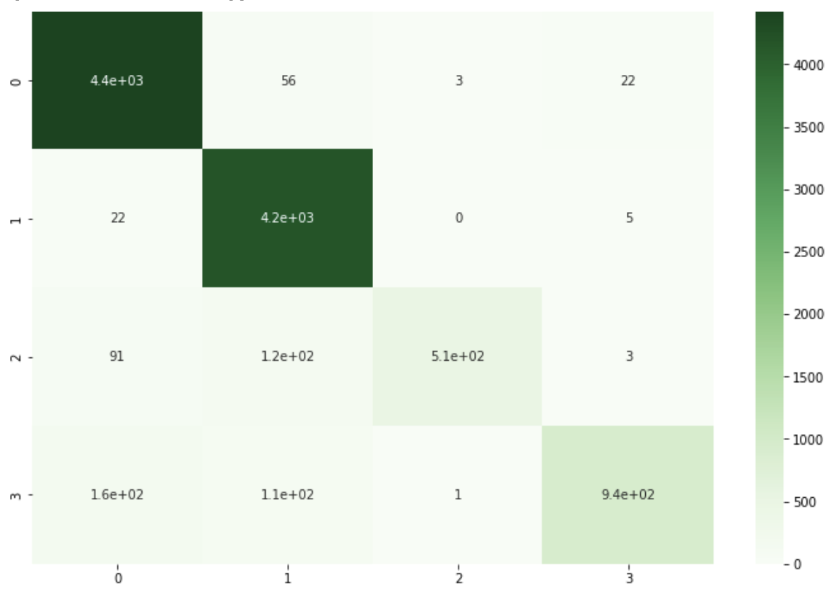
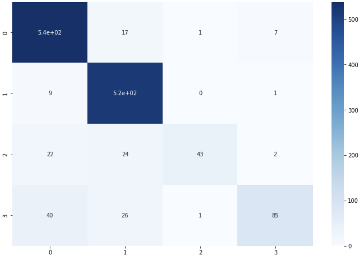
55. 混同行列の作成

52 で学習したロジスティック回帰モデルの混同行列（confusion matrix）を，学習データおよび評価データ上で作成せよ．

from sklearn.metrics import confusion_matrix
import seaborn as sns
import matplotlib.pyplot as plt

# train data
train_cm = confusion_matrix(train['CATEGORY'], y_pred_train)
print(train_cm)
plt.figure(figsize=(12, 8))
sns.heatmap(train_cm, annot=True, cmap='Greens')
plt.show()

[[4421   56    3   22]
 [  22 4196    0    5]
 [  91  125  509    3]
 [ 162  111    1  945]]

confusion matrix 55

# test data
test_cm = confusion_matrix(test['CATEGORY'], y_pred_test)
print(test_cm)
plt.figure(figsize=(12, 8))
sns.heatmap(test_cm, annot=True, cmap='Blues')
plt.show()

[[538  17   1   7]
 [  9 518   0   1]
 [ 22  24  43   2]
 [ 40  26   1  85]]

confusion matrix 55

56. 適合率，再現率，F1 スコアの計測

52 で学習したロジスティック回帰モデルの適合率，再現率，F1 スコアを，評価データ上で計測せよ．カテゴリごとに適合率，再現率，F1 スコアを求め，カテゴリごとの性能をマイクロ平均（micro-average）とマクロ平均（macro-average）で統合せよ．

from sklearn.metrics import precision_score, recall_score, f1_score
import numpy as np

# precision
precision = precision_score(test['CATEGORY'], y_pred_test, average=None, labels=model.classes_)
precision = np.append(precision, precision_score(test['CATEGORY'], y_pred_test, average='micro'))
precision = np.append(precision, precision_score(test['CATEGORY'], y_pred_test, average='macro'))

# recall
recall = recall_score(test['CATEGORY'], y_pred_test, average=None, labels=model.classes_)
recall = np.append(recall, recall_score(test['CATEGORY'], y_pred_test, average='micro'))
recall = np.append(recall, recall_score(test['CATEGORY'], y_pred_test, average='macro'))

# F1
f1 = f1_score(test['CATEGORY'], y_pred_test, average=None, labels=['b', 'e', 't', 'm'])
f1 = np.append(f1, f1_score(test['CATEGORY'], y_pred_test, average='micro'))
f1 = np.append(f1, f1_score(test['CATEGORY'], y_pred_test, average='macro'))

scores = pd.DataFrame({'precision': precision, 'recall': recall, 'F1': f1},
                    index=['b', 'e', 't', 'm', 'micro avg', 'macro avg'])

print(scores)

           precision    recall        f1
b           0.883415  0.955595  0.918089
e           0.885470  0.981061  0.930818
t           0.955556  0.472527  0.688259
m           0.894737  0.559211  0.632353
micro avg   0.887556  0.887556  0.887556
macro avg   0.904794  0.742098  0.792380

57. 特徴量の重みの確認

52 で学習したロジスティック回帰モデルの中で，重みの高い特徴量トップ 10 と，重みの低い特徴量トップ 10 を確認せよ．

features = x_train.columns.values
index = [i for i in range(1, 11)]
for c, coef in zip(model.classes_, model.coef_):
  print(f'category: {c}', '*' * 100)
  best_10 = pd.DataFrame(features[np.argsort(coef)[::-1][:10]], columns=['best 10'], index=index).T
  worst_10 = pd.DataFrame(features[np.argsort(coef)[:10]], columns=['worst 10'], index=index).T
  print(pd.concat([best_10, worst_10], axis=0))
  print('\n')

category: b ****************************************************************************************************
           1     2    3      4         5        6      7       8           9   \
best 10   fed  bank  ecb  china       oil  ukraine   euro  update      stocks
worst 10  and   the  her  ebola  facebook      she  video   study  kardashian

              10
best 10      buy
worst 10  google


category: e ****************************************************************************************************
                  1      2       3     4    5      6        7      8      9   \
best 10   kardashian  chris     kim   she  her  cyrus    miley   star   paul
worst 10      update     us  google  says  ceo  study  billion  china  could

                10
best 10      movie
worst 10  facebook


category: m ****************************************************************************************************
             1         2        3     4      5        6       7       8   \
best 10   ebola    cancer    study  drug    fda     mers  health   virus
worst 10     gm  facebook  climate   ceo  apple  twitter    deal  google

             9      10
best 10   could  heart
worst 10  sales    buy


category: t ****************************************************************************************************
              1         2      3        4          5         6        7   \
best 10   google  facebook  apple  climate  microsoft        gm  tmobile
worst 10     her        at   drug      fed        but  american   shares

               8           9       10
best 10   samsung  heartbleed   tesla
worst 10   cancer        bank  stocks

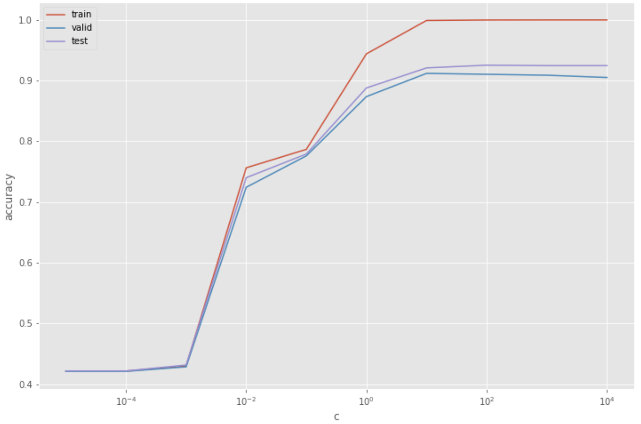
58. 正則化パラメータの変更

ロジスティック回帰モデルを学習するとき，正則化パラメータを調整することで，学習時の過学習（overfitting）の度合いを制御できる．異なる正則化パラメータでロジスティック回帰モデルを学習し，学習データ，検証データ，および評価データ上の正解率を求めよ．実験の結果は，正則化パラメータを横軸，正解率を縦軸としたグラフにまとめよ．

from tqdm import tqdm
import matplotlib.pyplot as plt

plt.style.use('ggplot')

c_list = np.logspace(-5, 4, 10, base=10)
# models = [LogisticRegression(C=C, random_state=42, max_iter=1000).fit(x_train, train['CATEGORY']) for C in tqdm(c_list)]

train_accs = [accuracy_score(model.predict(x_train), train['CATEGORY']) for model in models]
valid_accs = [accuracy_score(model.predict(x_valid), valid['CATEGORY']) for model in models]
test_accs = [accuracy_score(model.predict(x_test), test['CATEGORY']) for model in models]

plt.plot(c_list, train_accs, label = 'train')
plt.plot(c_list, valid_accs, label = 'valid')
plt.plot(c_list, test_accs, label = 'test')
plt.xscale('log')
plt.xlabel('c')
plt.ylabel('accuracy')
plt.legend()
plt.show()

59. ハイパーパラメータの探索

学習アルゴリズムや学習パラメータを変えながら，カテゴリ分類モデルを学習せよ．検証データ上の正解率がもっとも高くなる学習アルゴリズム・パラメータを求めよ．また，その学習アルゴリズム・パラメータを用いたときの評価データ上の正解率を求めよ．

!pip install optuna

import optuna

def objective(trial):
  model = LogisticRegression(random_state=42,
                             max_iter=10000,
                             penalty='elasticnet',
                             solver='saga',
                             l1_ratio=trial.suggest_uniform('l1_ratio', 0, 1),
                             C=trial.suggest_loguniform('C', 1e-4, 1e2))
  model.fit(x_train, train['CATEGORY'])
  valid_accuracy = accuracy_score(model.predict(x_valid), valid['CATEGORY'])

  return valid_accuracy

study = optuna.create_study(direction='maximize')
study.optimize(objective, n_trials=2, timeout=3600)

print('Best trial:')
trial = study.best_trial
print('  Value: {:.3f}'.format(trial.value))
print('  Params: ')
for key, value in trial.params.items():
  print('    {}: {}'.format(key, value))

>> Best trial:
>>   Value: 0.657
>>   Params:
>>     l1_ratio: 0.8173726339927334
>>     C: 0.08584685734174859

model = LogisticRegression(random_state=42,
                           max_iter=10000,
                           penalty='elasticnet',
                           solver='saga',
                           l1_ratio=trial.params['l1_ratio'],
                           C=trial.params['C'])
model.fit(x_train, train['CATEGORY'])

y_pred_train = model.predict(x_train)
y_pred_valid = model.predict(x_valid)
y_pred_test = model.predict(x_test)

train_accuracy = accuracy_score(train['CATEGORY'], y_pred_train)
valid_accuracy = accuracy_score(valid['CATEGORY'], y_pred_valid)
test_accuracy = accuracy_score(test['CATEGORY'], y_pred_test)

print(f'accuracy (train)：{train_accuracy:.3f}')
print(f'accuracy (valid)：{valid_accuracy:.3f}')
print(f'accuracy (test)：{test_accuracy:.3f}')

>> accuracy (train)：0.668
>> accuracy (valid)：0.657
>> accuracy (test)：0.653