2022-03-28

共分散

共分散とは

共分散とは、2つの変数XとYの関係を表す数値です。一方の変数が増加すると、もう一方の変数が増加または減少するかどうかを示します。

共分散が正である場合、両変数が共に増加または減少する傾向があることを示します。共分散が負である場合、一方の変数が増加すると、他方の変数が減少する傾向があることを示し、その逆も同様です。共分散がゼロの場合、変数間に線形関係がないことを意味します。

変数 $X$ と $Y$ の共分散の数学的表現は以下のとおりです。

cov(X,Y) = \frac{\sum_{i=1}^{n}(X_i-\overline{X})(Y_i-\overline{Y})}{n-1}

ここで、

$cov(X,Y)$ : 変数XとYの共分散
$X_i$ と $Y_i$ : 変数XとYの個々のデータポイント
$\overline{X}$ と $\overline{Y}$ : 変数XとYの平均値
$n$ : データポイントの数

共分散と相関の違い

共分散は2つの変数の関係の向きを測定するのに対し、相関はその関係の強さと向きを定量化します。相関は、-1から1までの範囲で標準化された共分散であり、共分散は任意の値を取ることができます。

相関係数は、以下のように計算されます。

r = \frac{cov(X,Y)}{\sigma_X\sigma_Y}

ここで、

$r$ ：相関係数
$cov(X,Y)$ ：変数XとYの共分散
$\sigma_X$ と $\sigma_Y$ ：変数XとYの標準偏差

Pythonで共分散を計算

この章では、Pythonを使用して共分散を計算する方法を説明し、正の共分散と負の共分散の両方の場合を示します。また、変数間の関係を視覚化するためのプロットも作成します。

まずは必要なライブラリをインポートします。

python

import numpy as np
import pandas as pd
import matplotlib.pyplot as plt
import seaborn as sns

次に、2つの変数の間の共分散を計算する関数を作成します。

python

def covariance(x, y):
    x_mean = np.mean(x)
    y_mean = np.mean(y)
    n = len(x)
    cov = np.sum((x - x_mean) * (y - y_mean)) / (n - 1)
    return cov

正の共分散の例を作成してみます。

python

# Generate sample data with positive covariance
np.random.seed(42)
x_positive = np.random.rand(50)
y_positive = x_positive * 3 + np.random.rand(50)

# Calculate the covariance
positive_cov = covariance(x_positive, y_positive)
print(f"Positive Covariance: {positive_cov}")

# Plot the data
plt.figure(figsize=(10, 6))
sns.set(style="whitegrid")
sns.scatterplot(x=x_positive, y=y_positive, s=100, color="blue", edgecolor="black")
plt.title("Positive Covariance Example", fontsize=20)
plt.xlabel("X", fontsize=16)
plt.ylabel("Y", fontsize=16)
plt.show()

Positive Covariance: 0.25587483932859534

Positive covariance

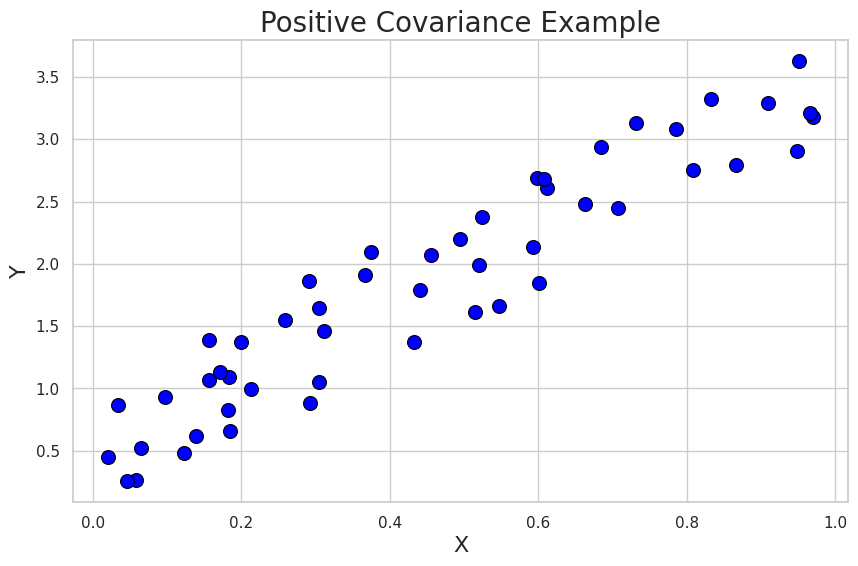
この例では、Xの値が増加すると、Yの値も増加する傾向があることがわかります。プロットは、変数間の正の共分散を示しています。

次に、負の共分散の例を作成してみます。

python

# Generate sample data with negative covariance
np.random.seed(42)
x_negative = np.random.rand(50)
y_negative = -x_negative * 3 + np.random.rand(50)

# Calculate the covariance
negative_cov = covariance(x_negative, y_negative)
print(f"Negative Covariance: {negative_cov}")

# Plot the data
plt.figure(figsize=(10, 6))
sns.set(style="whitegrid")
sns.scatterplot(x=x_negative, y=y_negative, s=100, color="red", edgecolor="black")
plt.title("Negative Covariance Example", fontsize=20)
plt.xlabel("X", fontsize=16)
plt.ylabel("Y", fontsize=16)
plt.show()

Negative Covariance: -0.2448461835209279

Negative covariance

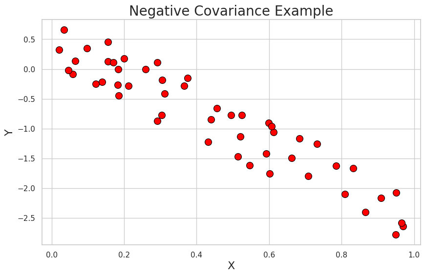
この例では、Xの値が増加すると、Yの値が減少する傾向があることがわかります。プロットは、変数間の負の共分散を示しています。

共分散

共分散とは

共分散と相関の違い

Pythonで共分散を計算

Zスコア

相関係数

Ryusei Kakujo