


What is standard normal distribution table
The Standard Normal Distribution Table is a table that calculates the area of a normal distribution with mean 0 and variance 1. The standard normal distribution table includes the following graph and number table.
| z | 0 | 0.01 | 0.02 | 0.03 | 0.04 | 0.05 | 0.06 | 0.07 | 0.08 | 0.09 |
|---|---|---|---|---|---|---|---|---|---|---|
| 0 | 0 | 0.003989 | 0.007978 | 0.011966 | 0.015953 | 0.019939 | 0.023922 | 0.027903 | 0.031881 | 0.035856 |
| 0.1 | 0.039828 | 0.043795 | 0.047758 | 0.051717 | 0.055670 | 0.059618 | 0.063559 | 0.067495 | 0.071424 | 0.075345 |
| 0.2 | 0.079260 | 0.083166 | 0.087064 | 0.090954 | 0.094835 | 0.098706 | 0.102568 | 0.106420 | 0.110261 | 0.114092 |
| 0.3 | 0.117911 | 0.121720 | 0.125516 | 0.129300 | 0.133072 | 0.136831 | 0.140576 | 0.144309 | 0.148027 | 0.151732 |
| 0.4 | 0.155422 | 0.159097 | 0.162757 | 0.166402 | 0.170031 | 0.173645 | 0.177242 | 0.180822 | 0.184386 | 0.187933 |
| 0.5 | 0.191462 | 0.194974 | 0.198468 | 0.201944 | 0.205401 | 0.208840 | 0.212260 | 0.215661 | 0.219043 | 0.222405 |
| 0.6 | 0.225747 | 0.229069 | 0.232371 | 0.235653 | 0.238914 | 0.242154 | 0.245373 | 0.248571 | 0.251748 | 0.254903 |
| 0.7 | 0.258036 | 0.261148 | 0.264238 | 0.267305 | 0.270350 | 0.273373 | 0.276373 | 0.279350 | 0.282305 | 0.285236 |
| 0.8 | 0.288145 | 0.291030 | 0.293892 | 0.296731 | 0.299546 | 0.302337 | 0.305105 | 0.307850 | 0.310570 | 0.313267 |
| 0.9 | 0.315940 | 0.318589 | 0.321214 | 0.323814 | 0.326391 | 0.328944 | 0.331472 | 0.333977 | 0.336457 | 0.338913 |
| 1.0 | 0.341345 | 0.343752 | 0.346136 | 0.348495 | 0.350830 | 0.353141 | 0.355428 | 0.357690 | 0.359929 | 0.362143 |
| 1.1 | 0.364334 | 0.366500 | 0.368643 | 0.370762 | 0.372857 | 0.374928 | 0.376976 | 0.379000 | 0.381000 | 0.382977 |
| 1.2 | 0.384930 | 0.386861 | 0.388768 | 0.390651 | 0.392512 | 0.394350 | 0.396165 | 0.397958 | 0.399727 | 0.401475 |
| 1.3 | 0.403200 | 0.404902 | 0.406582 | 0.408241 | 0.409877 | 0.411492 | 0.413085 | 0.414657 | 0.416207 | 0.417736 |
| 1.4 | 0.419243 | 0.420730 | 0.422196 | 0.423641 | 0.425066 | 0.426471 | 0.427855 | 0.429219 | 0.430563 | 0.431888 |
| 1.5 | 0.433193 | 0.434478 | 0.435745 | 0.436992 | 0.438220 | 0.439429 | 0.440620 | 0.441792 | 0.442947 | 0.444083 |
| 1.6 | 0.445201 | 0.446301 | 0.447384 | 0.448449 | 0.449497 | 0.450529 | 0.451543 | 0.452540 | 0.453521 | 0.454486 |
| 1.7 | 0.455435 | 0.456367 | 0.457284 | 0.458185 | 0.459070 | 0.459941 | 0.460796 | 0.461636 | 0.462462 | 0.463273 |
| 1.8 | 0.464070 | 0.464852 | 0.465620 | 0.466375 | 0.467116 | 0.467843 | 0.468557 | 0.469258 | 0.469946 | 0.470621 |
| 1.9 | 0.471283 | 0.471933 | 0.472571 | 0.473197 | 0.473810 | 0.474412 | 0.475002 | 0.475581 | 0.476148 | 0.476705 |
| 2.0 | 0.477250 | 0.477784 | 0.478308 | 0.478822 | 0.479325 | 0.479818 | 0.480301 | 0.480774 | 0.481237 | 0.481691 |
| 2.1 | 0.482136 | 0.482571 | 0.482997 | 0.483414 | 0.483823 | 0.484222 | 0.484614 | 0.484997 | 0.485371 | 0.485738 |
| 2.2 | 0.486097 | 0.486447 | 0.486791 | 0.487126 | 0.487455 | 0.487776 | 0.488089 | 0.488396 | 0.488696 | 0.488989 |
| 2.3 | 0.489276 | 0.489556 | 0.489830 | 0.490097 | 0.490358 | 0.490613 | 0.490863 | 0.491106 | 0.491344 | 0.491576 |
| 2.4 | 0.491802 | 0.492024 | 0.492240 | 0.492451 | 0.492656 | 0.492857 | 0.493053 | 0.493244 | 0.493431 | 0.493613 |
| 2.5 | 0.493790 | 0.493963 | 0.494132 | 0.494297 | 0.494457 | 0.494614 | 0.494766 | 0.494915 | 0.495060 | 0.495201 |
| 2.6 | 0.495339 | 0.495473 | 0.495604 | 0.495731 | 0.495855 | 0.495975 | 0.496093 | 0.496207 | 0.496319 | 0.496427 |
| 2.7 | 0.496533 | 0.496636 | 0.496736 | 0.496833 | 0.496928 | 0.497020 | 0.497110 | 0.497197 | 0.497282 | 0.497365 |
| 2.8 | 0.497445 | 0.497523 | 0.497599 | 0.497673 | 0.497744 | 0.497814 | 0.497882 | 0.497948 | 0.498012 | 0.498074 |
| 2.9 | 0.498134 | 0.498193 | 0.498250 | 0.498305 | 0.498359 | 0.498411 | 0.498462 | 0.498511 | 0.498559 | 0.498605 |
| 3.0 | 0.498650 | 0.498694 | 0.498736 | 0.498777 | 0.498817 | 0.498856 | 0.498893 | 0.498930 | 0.498965 | 0.498999 |
| 3.1 | 0.499032 | 0.499065 | 0.499096 | 0.499126 | 0.499155 | 0.499184 | 0.499211 | 0.499238 | 0.499264 | 0.499289 |
| 3.2 | 0.499313 | 0.499336 | 0.499359 | 0.499381 | 0.499402 | 0.499423 | 0.499443 | 0.499462 | 0.499481 | 0.499499 |
| 3.3 | 0.499517 | 0.499534 | 0.499550 | 0.499566 | 0.499581 | 0.499596 | 0.499610 | 0.499624 | 0.499638 | 0.499651 |
| 3.4 | 0.499663 | 0.499675 | 0.499687 | 0.499698 | 0.499709 | 0.499720 | 0.499730 | 0.499740 | 0.499749 | 0.499758 |
| 3.5 | 0.499767 | 0.499776 | 0.499784 | 0.499792 | 0.499800 | 0.499807 | 0.499815 | 0.499822 | 0.499828 | 0.499835 |
| 3.6 | 0.499841 | 0.499847 | 0.499853 | 0.499858 | 0.499864 | 0.499869 | 0.499874 | 0.499879 | 0.499883 | 0.499888 |
| 3.7 | 0.499892 | 0.499896 | 0.499900 | 0.499904 | 0.499908 | 0.499912 | 0.499915 | 0.499918 | 0.499922 | 0.499925 |
| 3.8 | 0.499928 | 0.499931 | 0.499933 | 0.499936 | 0.499938 | 0.499941 | 0.499943 | 0.499946 | 0.499948 | 0.499950 |
| 3.9 | 0.499952 | 0.499954 | 0.499956 | 0.499958 | 0.499959 | 0.499961 | 0.499963 | 0.499964 | 0.499966 | 0.499967 |
| 4.0 | 0.499968 | 0.499970 | 0.499971 | 0.499972 | 0.499973 | 0.499974 | 0.499975 | 0.499976 | 0.499977 | 0.499978 |
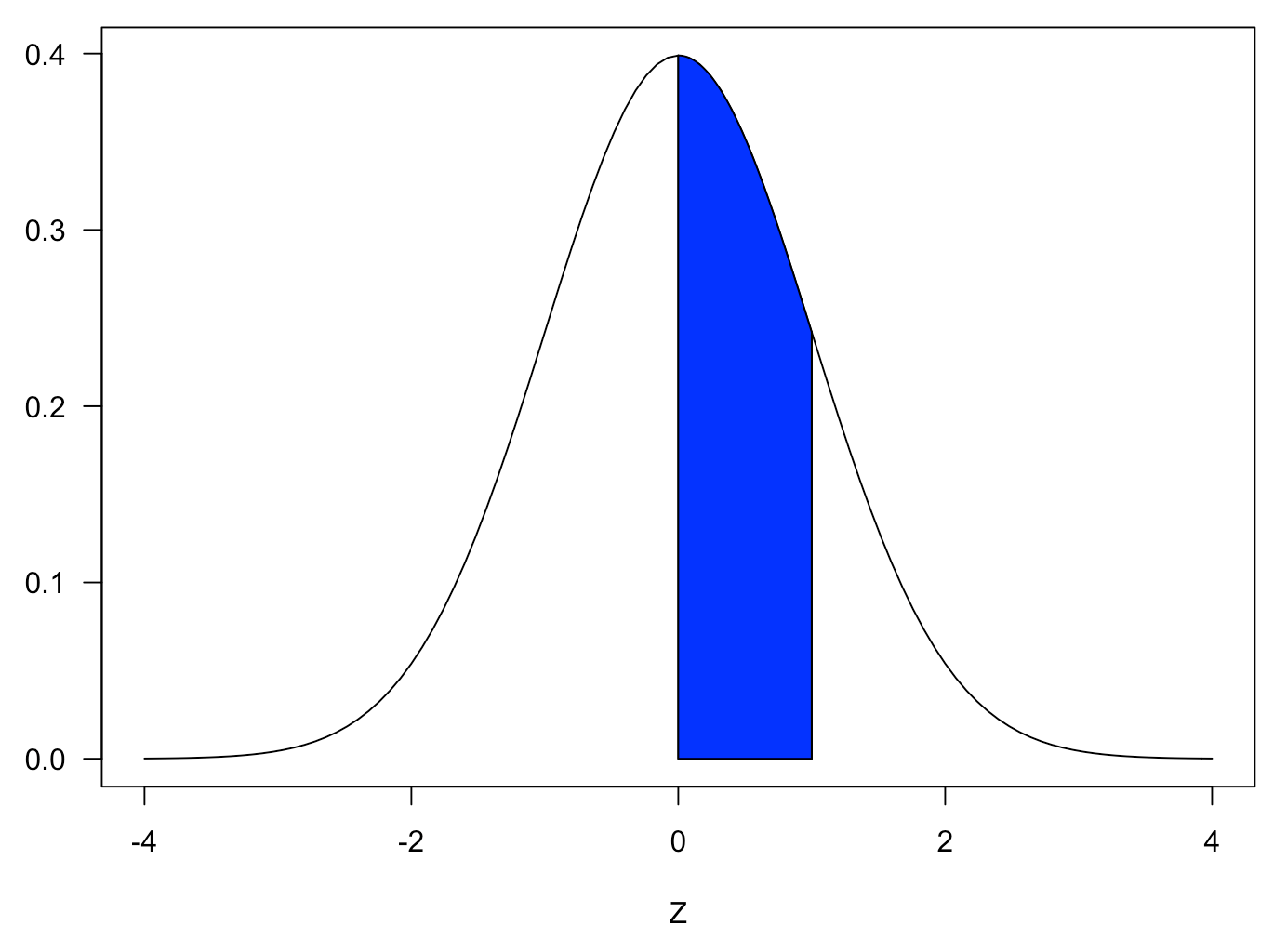
The number table shows the result of calculating the blue area of the graph. The horizontal axis of the graph is a value called the z-value.
What is a z-value
Any normal distribution can be standardized and converted to a standard normal distribution. z-value is a value that standardizes the normal distribution and indicates how many standard deviations the data are from the mean.
If the mean of a normal distribution is
How to create a standard normal distribution table
This time, we will create a standard normal distribution table in Google Sheets to calculate the blue area in the figure below.
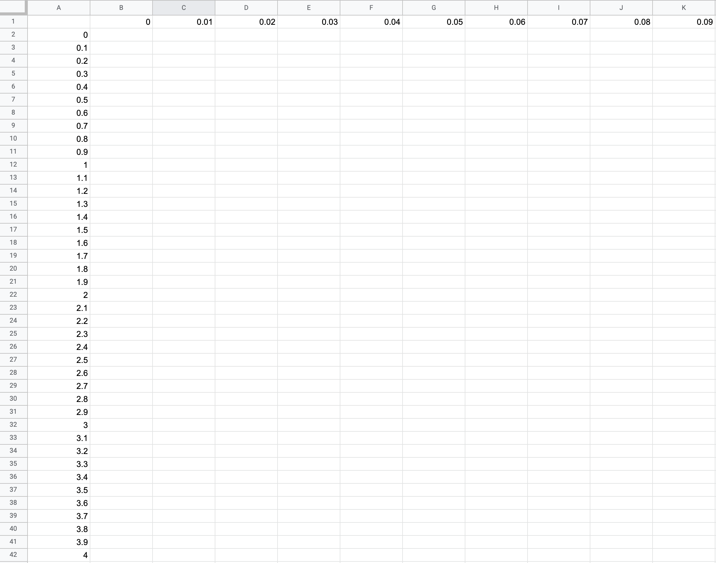
First, fill in column A and row 1 of Google Sheets as follows.
Then enter the function =NORM.DIST($A2+B$1,0,1,TRUE)-0.5 in cell B2.
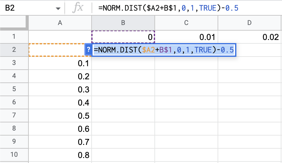
Drag cell B2 to reflect the function throughout the table.
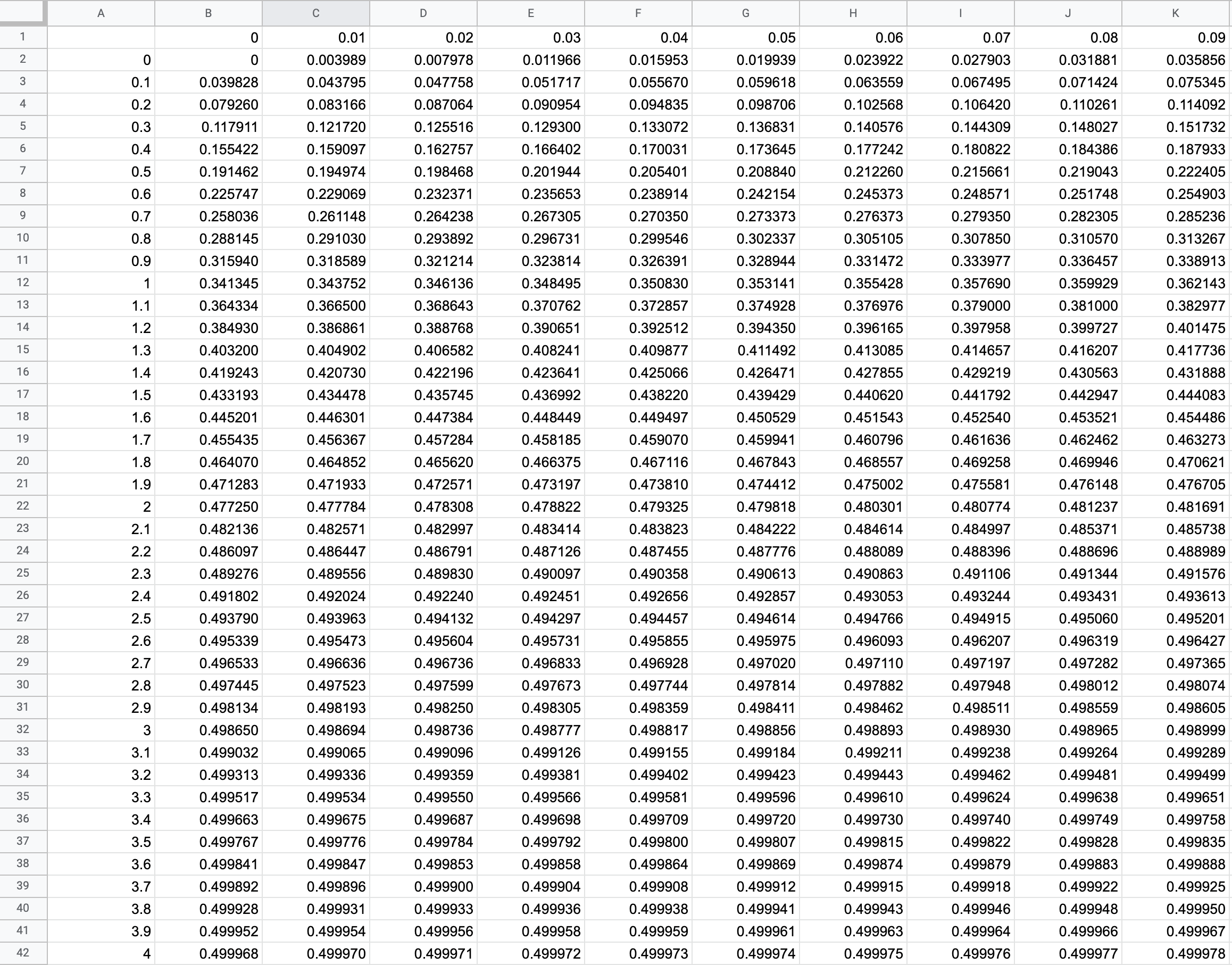
This completes the standard normal distribution table.
The function NORM.DIST() used as a function calculates the area of the normal distribution, and its argument is NORM.DIST(𝑥, mean, standard deviation, function form). The following green area is calculated.
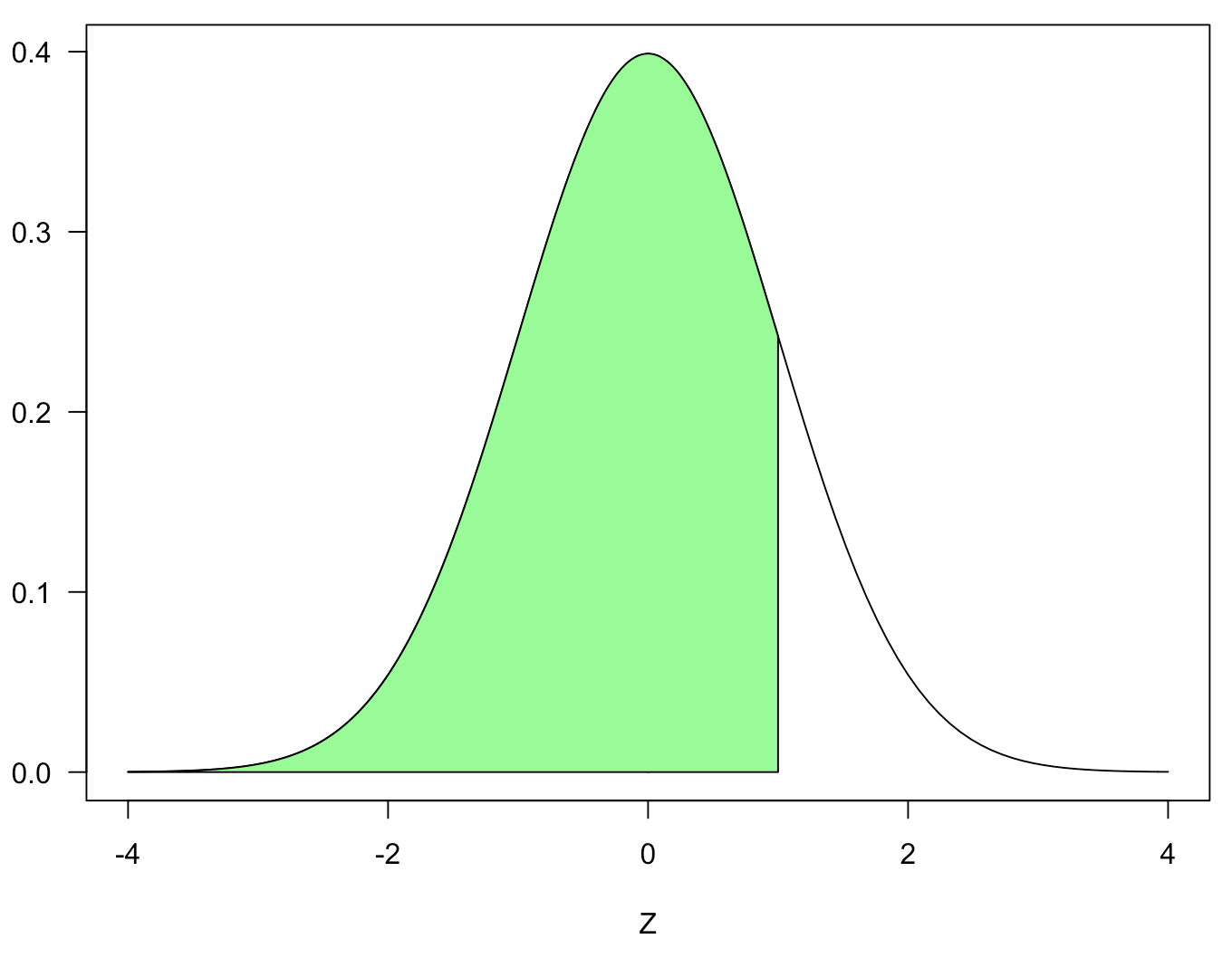
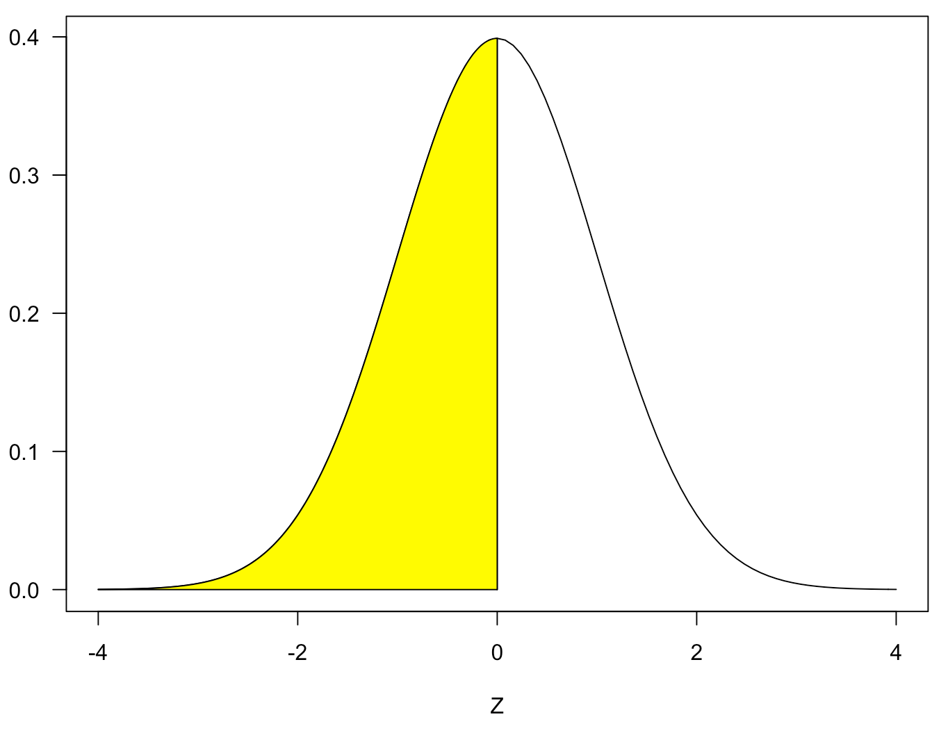
Therefore, to calculate the area of the target (blue), subtract the yellow area in the figure below from the green area. The area of the yellow portion is 0.5, so the function will be NORM.DIST()-0.5.
The R code used to draw the normal distribution is shown below.
# green area
curve(dnorm(x), -4, 4, las=1, xlab="Z")
arrows(0,0,0,dnorm(0),length=0)
xvalu <- seq(-4,1,length=200)
dvalu <- dnorm(xvalu)
polygon(c(xvalu, rev(xvalu)), c(rep(0,200), rev(dvalu)),col="palegreen")

# yellow area
curve(dnorm(x), -4, 4, las=1, xlab="Z")
arrows(0,0,0,dnorm(0),length=0)
xvalu <- seq(-4,0,length=200)
dvalu <- dnorm(xvalu)
polygon(c(xvalu, rev(xvalu)), c(rep(0,200), rev(dvalu)),col="yellow")

# blue area
curve(dnorm(x), -4, 4, las=1, xlab="Z")
arrows(0,0,0,dnorm(0),length=0)
xvalu <- seq(0,1,length=200)
dvalu <- dnorm(xvalu)
polygon(c(xvalu, rev(xvalu)), c(rep(0,200), rev(dvalu)),col="blue")
How to read the standard normal distribution table
The following is a flowchart of how to read the standard normal distribution table.
- Find the row of numbers with one place and one decimal place 2.
- Find the column of numbers to the second decimal place 3.
- Read the number at the intersection of the two.
Let us read from the standard normal distribution table if the z-value is 1.96. First, find the matrix where the first place and the first decimal place are 1.9.
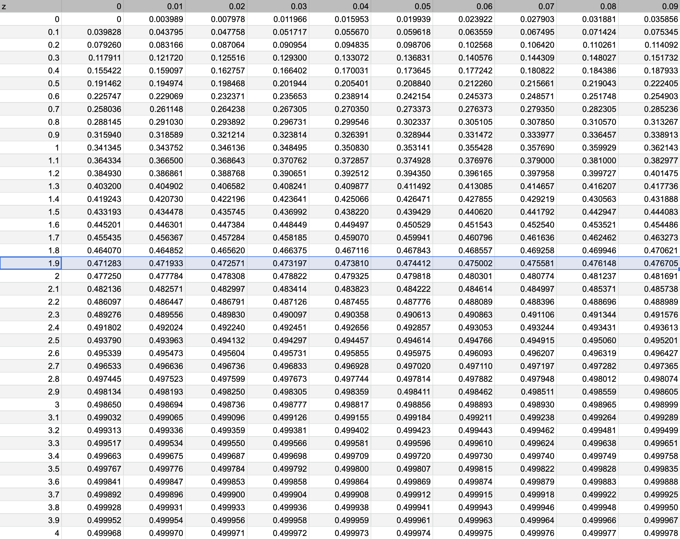
Next, find the column with the second decimal place of 0.06.
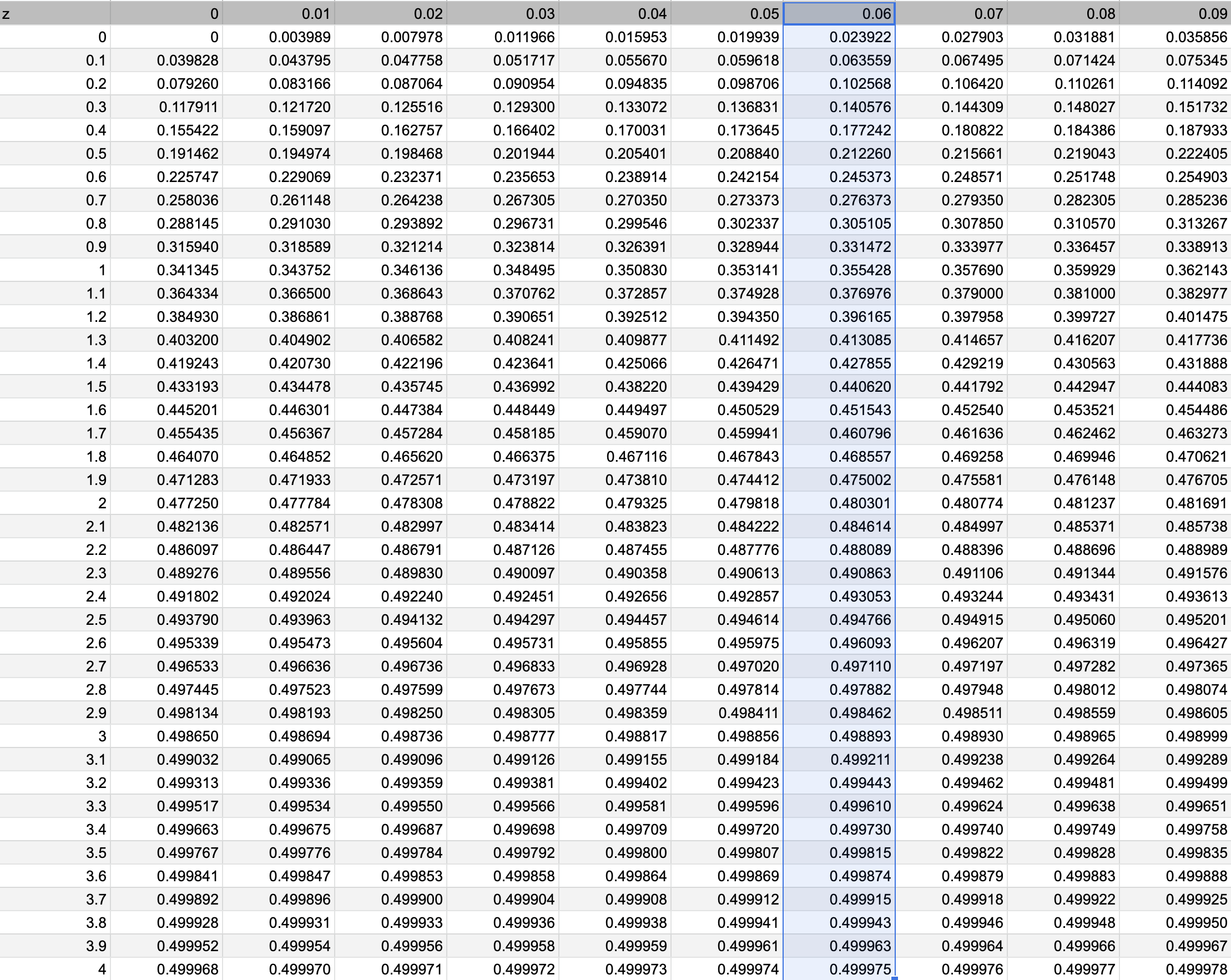
The value at the intersection of the two is 0.475002, indicating that there is a 47.5% probability that z=1.96.


Ryusei Kakujo


Weave the future of cities through data
Transportation modeling/ Urban planning/ Machine learning/ Computer science/ GIS