Introduction

When several statistical models are created, this article describes the AIC, which is one indicator as to which statistical model can be considered a good model.

Data and Models

In this article, I will use the seed count data and the statistical model for 100 fictitious plants, which were treated in the article Generalized linear model.

The data are as follows: y is the number of seeds per individual, x is the size of the individual, and f is whether the individual has been treated with fertilizer or not (categorical variable).

From this data, the following Poisson regression models have been constructed:

• Statistical model where the number of seeds depends on the size (x model)
  • \lambda_i = e^{\beta_1 + \beta_2 x_i}
• Statistical model in which the number of seeds depends on the presence or absence of fertilizer treatments (f model)
  • \lambda_i = e^{\beta_1 + \beta_3 d_i} (d_i is a dummy variable)
• Statistical model where seed number depends on size and fertilizer treatment (xf model)
  • \lambda_i = e^{\beta_1 + \beta_2 x_i + \beta_3 d_i} (d_i is a dummy variable)

Deviance

We have searched for parameters that maximize the log-likelihood, which is the goodness of fit to the observed data, when the parameters of the statistical model are estimated by maximum likelihood.

Here, there is a measure called deviance that indicates the poor fit. The deviance D is defined by the following equation:

The \log L^* is the maximum log-likelihood. The actual deviance is just the maximum log-likelihood \log L^* multiplied by -2.

A summary of the parameter estimation results for the x model is shown below.

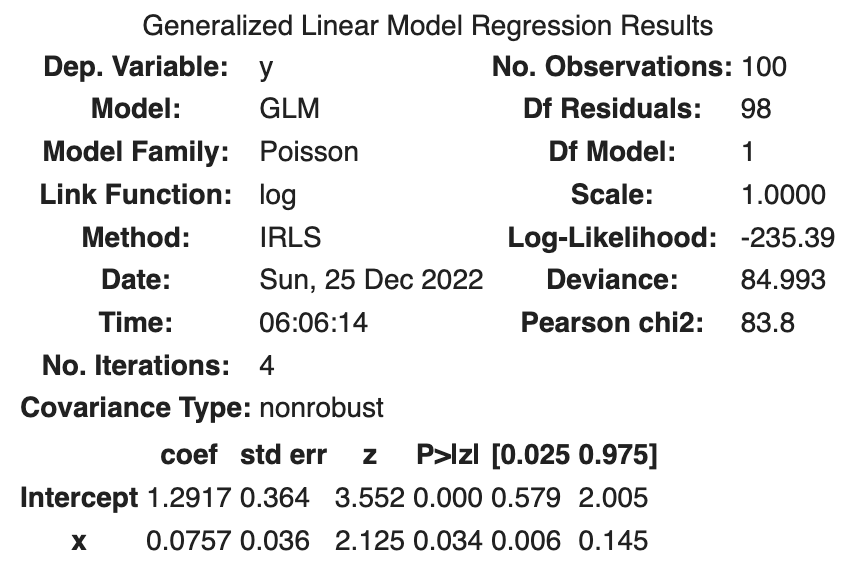
The maximum log likelihood is -235.39, so the deviance D = \log L^*$ is 470.78. However, the value 470.78 is not shown in the summary, but instead the value Deviance is shown.

The Deviance shown is the residual deviance, which is defined as follows.

The D_{min} is the deviation from the full model. A full model is a model fitted with a number of parameters corresponding to the number of data. For example, since the number of data in this case is 100, it is a statistical model fitted with 100 parameters. In other words, the full model is not valuable as a statistical model since it only reads out all the data. However, the full model has the maximum goodness of fit, or log-likelihood, and the minimum deviance D_{min}.

The residual deviance is the relative value of the poor fit with respect to the deviance of the full model.

Next, we consider the maximum residual deviance. The model with the maximum deviation is the model with the worst fit, i.e., the model with no explanatory variables incorporated. This model is called the Null model.

The Null model can be constructed as follows.

import statsmodels.api as sm
import statsmodels.formula.api as smf

fit_null = smf.glm('y ~ 1', data=df, family=sm.families.Poisson()).fit()
fit_null.summary()

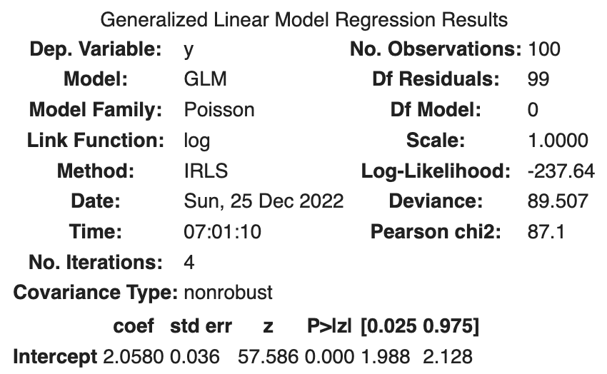
The maximum residual deviance D_{max} is 89.507.

The following table summarizes the deviations.

The following is a summary of each model.

It can be seen that the model with a larger number of parameters fits the data better.

AIC

We have seen that increasing the complexity of the model, i.e., increasing the number of parameters in the model, improves the maximum log-likelihood and improves the fit to the observed data. However, it may only be a good fit for the observed data obtained by chance, and may not be a good fit at all for other data. In other words, it may be good for one set of observations, but poor for another set of observations. In machine learning terms, this means that you may be over-training on the training data.

AIC is a measure that emphasizes good prediction rather than goodness of fit.

The AIC is expressed by the following equation:

k is the number of parameters estimated by maximum likelihood. The smaller the AIC, the better the model.

The AIC is easily output by the following code.

print('null model', fit_null.aic)
print('f model', fit_f.aic)
print('x model', fit_x.aic)

null model 477.2864426185736
f model 479.25451392137364
x model 477.2864426185736

Using AIC as the criterion, the x model is the best model.

Notes on model selection by AIC

If there are few observed data, a model with fewer parameters may have a smaller AIC than the true model. A simple model may have better predictive power because the observed data is too small to find a rule of thumb in the data.