2022-11-20

What is regression analysis

What is regression analysis?

Regression analysis is a statistical technique that expresses causal relationships as a function of which factors influence which outcome and by how much. In this case, the numerical value that is the outcome is called the objective variable and the numerical value that is the factor is called the explanatory variable.

When there is only one explanatory variable, it is called simple regression analysis, and when there are multiple explanatory variables, it is called multiple regression analysis.

Regression analysis is a widely used statistical technique in both business and academia.

Examples of regression analysis

The following are examples of regression analysis.

Prediction of real estate prices
- Simple Regression Analysis
  - Objective variable: real estate prices
  - Explanatory variable: lot size
- Multiple regression analysis
  - Objective variable: real estate price
  - Explanatory variables: lot size, distance from station, age of building, etc.
Prediction of click rate on advertisements
- Simple regression analysis
  - Objective variable: click rate
  - Explanatory variable: title
- Multiple regression analysis
  - Objective variable: click rate
  - Explanatory variables: title, font, genre, etc.

Regression analysis in Python

Here is the code to implement regression analysis in Python. In this case, I will use Boston home price data from sklearn as the dataset.

import pandas as pd
from sklearn import datasets

boston = datasets.load_boston()
df = pd.DataFrame(boston.data, columns=boston.feature_names)
df["PRICE"] = boston.target
df.head()

Linear regression | 1

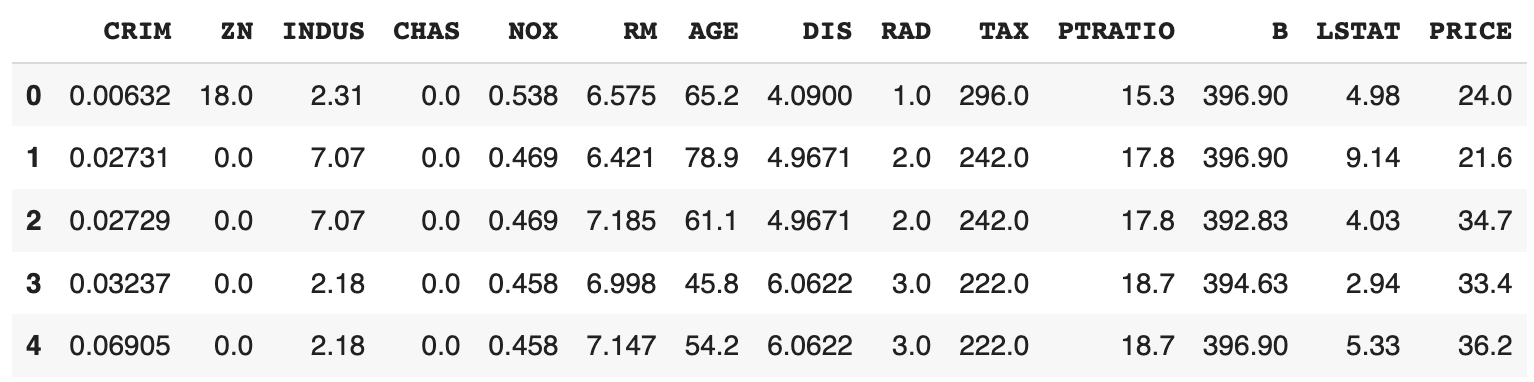
The PRICE label is the house price and the rest of the labels are data on the characteristics of the house.

Details of the labels in each column can be seen by DESCR.

print(boston.DESCR)

.. _boston_dataset:

Boston house prices dataset
---------------------------

**Data Set Characteristics:**

    :Number of Instances: 506

    :Number of Attributes: 13 numeric/categorical predictive. Median Value (attribute 14) is usually the target.

    :Attribute Information (in order):
        - CRIM     per capita crime rate by town
        - ZN       proportion of residential land zoned for lots over 25,000 sq.ft.
        - INDUS    proportion of non-retail business acres per town
        - CHAS     Charles River dummy variable (= 1 if tract bounds river; 0 otherwise)
        - NOX      nitric oxides concentration (parts per 10 million)
        - RM       average number of rooms per dwelling
        - AGE      proportion of owner-occupied units built prior to 1940
        - DIS      weighted distances to five Boston employment centres
        - RAD      index of accessibility to radial highways
        - TAX      full-value property-tax rate per $10,000
        - PTRATIO  pupil-teacher ratio by town
        - B        1000(Bk - 0.63)^2 where Bk is the proportion of black people by town
        - LSTAT    % lower status of the population
        - MEDV     Median value of owner-occupied homes in $1000's

    :Missing Attribute Values: None

    :Creator: Harrison, D. and Rubinfeld, D.L.

This is a copy of UCI ML housing dataset.
https://archive.ics.uci.edu/ml/machine-learning-databases/housing/


This dataset was taken from the StatLib library which is maintained at Carnegie Mellon University.

The Boston house-price data of Harrison, D. and Rubinfeld, D.L. 'Hedonic
prices and the demand for clean air', J. Environ. Economics & Management,
vol.5, 81-102, 1978.   Used in Belsley, Kuh & Welsch, 'Regression diagnostics
...', Wiley, 1980.   N.B. Various transformations are used in the table on
pages 244-261 of the latter.

The Boston house-price data has been used in many machine learning papers that address regression
problems.

.. topic:: References

   - Belsley, Kuh & Welsch, 'Regression diagnostics: Identifying Influential Data and Sources of Collinearity', Wiley, 1980. 244-261.
   - Quinlan,R. (1993). Combining Instance-Based and Model-Based Learning. In Proceedings on the Tenth International Conference of Machine Learning, 236-243, University of Massachusetts, Amherst. Morgan Kaufmann.

Split the data set into training and test data.

from sklearn.model_selection import train_test_split

x_train, x_test, y_train, y_test = train_test_split(
  boston.data,
  boston.target,
  random_state=0
)

Simple regression analysis

In simple regression analysis, one explanatory variable predicts the objective variable. Assuming $x$ as the explanatory variable, $y$ as the objective variable, $a$ as the coefficient, and $b$ as the intercept, the single regression model can be expressed as follows

y = ax + b

We will use python's sklearn to compute $a$ and $b$ . In this case, we will use the label RM in the dataset as the explanatory variable.

from sklearn import linear_model

x_rm_train = x_train[:, [5]]
x_rm_test = x_test[:, [5]]

model = linear_model.LinearRegression()
model.fit(x_train_rm, y_train)
a = model.coef_
b = model.intercept_
print("a: ", a)
print("b: ", b)

a:  [9.31294923]
b:  -36.180992646339206

Visualize the data and model.

import matplotlib.pyplot as plt

plt.scatter(x_rm_train, y_train, label="Train")
plt.scatter(x_rm_test, y_test, label="Test")

y_pred = model.predict(x_rm_train)
plt.plot(x_rm_train, y_pred, c="black")

plt.xlabel("RM")
plt.ylabel("PRICE")
plt.legend()
plt.show()

Linear regression | 2

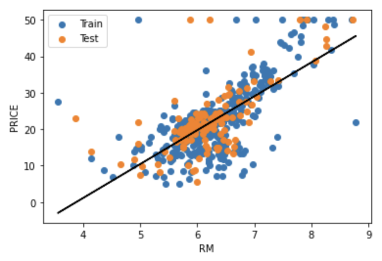
Train is the training data, Test is the test data, and the black line is the model.

Coefficient of determination

Calculates the coefficient of determination $R^2$ of the model. The $R^2$ takes values between 0 and 1. When $R^2$ is close to 1, it means that the predictions closely match the actual values. On the other hand, if $R^2$ is close to 0, it means that the model has very low predictive power.

The $R^2$ is represented by the following equation

R^2 = 1-{\frac {\displaystyle \sum _{i=1}^{N}\left(y_{i}-f_{i}\right)^{2}}{\displaystyle \sum _{j=1}^{N}\left(y_{j}-{\overline {y}}\right)^{2}}}

where $y_{i}$ is the correct values, $f_{i}$ is the predicted values, and ${\overline {y}}$ is the average of the correct values.

The $R^2$ can be easily computed with sklearn's r2_score function. The following code computes $R^2$ for each of the training and test data.

from sklearn.metrics import r2_score

y_pred_train = model.predict(x_rm_train)
print("R2 (train): ", r2_score(y_train, y_pred_train))

y_pred_test = model.predict(x_rm_test)
print("R2 (test): ", r2_score(y_test, y_pred_test))

R2 (train): 0.48752067939343646
R2 (test): 0.4679000543136781

MSE

Calculate the Mean Squared Error (MSE) of the model, where $E$ is the error, $y_k$ is the predicted value, and $t_k$ is the correct value, expressed as follows

E = \frac{1}{n} \sum_{k=1}^n(y_k-t_k)^2

A smaller MSE can be interpreted as a smaller error in the model.

The following code calculates the MSE for training and test data, respectively.

from sklearn.metrics import mean_squared_error

print("MSE (train): ", mean_squared_error(y_train, y_pred_train))

print("MSE (test): ", mean_squared_error(y_test, y_pred_test))

MSE (train):  43.71870658739849
MSE (test):  43.472041677202206

Multiple regression analysis

Multiple regression analysis predicts an objective variable with multiple explanatory variables. The multiple regression model is represented by the following equation with $x_k$ as each explanatory variable.

y = \sum_{k=1}^na_kx_k + b

This time, we will perform a multiple regression analysis using all the explanatory variables.

model = linear_model.LinearRegression()

model.fit(x_train, t_train)

a_df = pd.DataFrame(boston.feature_names, columns=["Exp"])
a_df["a"] = pd.Series(model.coef_)
a_df

	Exp	a
0	CRIM	-0.117735
1	ZN	0.044017
2	INDUS	-0.005768
3	CHAS	2.393416
4	NOX	-15.589421
5	RM	3.768968
6	AGE	-0.007035
7	DIS	-1.434956
8	RAD	0.240081
9	TAX	-0.011297
10	PTRATIO	-0.985547
11	B	0.008444
12	LSTAT	-0.499117

print("b: ", model.intercept_)

b:  36.93325545712031

Coefficient of Determination

Calculate the coefficient of determination for each of the training and test data.

from sklearn.metrics import r2_score

y_pred_train = model.predict(x_rm_train)
print("R2 (train): ", r2_score(y_train, y_pred_train))

y_pred_test = model.predict(x_rm_test)
print("R2 (test): ", r2_score(y_test, y_pred_test))

R2 (train): 0.7697699488741149
R2 (test): 0.635463843320211

Compared to the simple regression model, $R^2$ approaches 1, improving the agreement of the predictions with the correct values.

MSE

Calculate MSE on each of the training and test data.

from sklearn.metrics import mean_squared_error

print("MSE (train): ", mean_squared_error(y_train, y_pred_train))

print("MSE (test): ", mean_squared_error(y_test, y_pred_test))

MSE (train):  19.640519427908046
MSE (test):  29.78224509230252

The MSE was smaller compared to the simple regression model. However, the MSE for the test data was significantly larger than the MSE for the training data. In other words, the model may have over-fitted the training data. Thus, the goodness of the model should be judged not only in terms of $R^2$ and MSE improvement, but also with an awareness of the error divergence between the training data and the test data.