2023-01-27

DistilBERTでテキスト分類

Machine Learning

NLP

BERT

Python

はじめに

テキストの分類はNLPにおける一般的なタスクの一つであり、幅広い用途に利用することができます。この記事では、DistilBERT を使ってテキスト分類の一つである感情分析を行います。

Hugging Face のエコシステム

Hugging Face のエコシステムを使うと、生テキストから推論用にファインチューニングされたモデルを簡単に開発することができます。

Hugging Faceエコシステムにはコアとなる以下の3つのライブラリがあります。

Datasets
Tokenizers
Transformers

Hugging Faceエコシステムを使うと以下のようなフローで開発が進行します。

データセットの取得
解きたいタスクのためのデータセットをHugging Faceのページから検索（良さそうなデータセットが見当たらなければデータセットを自作）
Tokenizer の取得
Tokenizerは事前学習モデルに合ったものを取得
トークン化
データセットをTokenizerで処理
モデルの取得
事前学習モデルを取得
トレーニング
トレーニングの実行
推論
モデルの推論

以下では、上記のフローに従って、Google Colab環境でモデルを開発します。

ライブラリのインストール

以下のライブラリをインストールします。

!pip install transformers
!pip install datasets

データセットの取得

使用するデータセットをまず探す必要があります。

Hugging Faceは豊富なデータセットを提供しています。データセットは以下のリンクから検索することができます。

https://huggingface.co/datasets

Hugging Face Hubからデータをダウンロードするには、datasetsライブラリを使用します。この記事では、emotionというデータセットをダウンロードします。

from datasets import load_dataset

dataset = load_dataset("emotion")

取得したデータセットの中身を確認します。

>> dataset

DatasetDict({
    train: Dataset({
        features: ['text', 'label'],
        num_rows: 16000
    })
    validation: Dataset({
        features: ['text', 'label'],
        num_rows: 2000
    })
    test: Dataset({
        features: ['text', 'label'],
        num_rows: 2000
    })
})

データセットはtrain、 validation、 testに分かれており、それぞれがtextやlabelといった情報を持っていることが分かります。

取得したデータセットはフォーマットをpandasに設定することで、DataFrameとして扱うこともできます。

dataset.set_format(type="pandas")
train_df = dataset["train"][:]

>> train_df.head(5)

|     | text                                              | label |
| --- | ------------------------------------------------- | ----- |
| 0   | i didnt feel humiliated                           | 0     |
| 1   | i can go from feeling so hopeless to so damned... | 0     |
| 2   | im grabbing a minute to post i feel greedy wrong  | 3     |
| 3   | i am ever feeling nostalgic about the fireplac... | 2     |
| 4   | i am feeling grouchy                              | 3     |

labelの内訳を確認します。

>> train_df.value_counts(["label"])

label
1        5362
0        4666
3        2159
4        1937
2        1304
5         572
dtype: int64

6種類のラベルが存在することが分かります。各ラベルの意味はfeaturesを使うと確認することができます。

>> dataset["train"].features

{'text': Value(dtype='string', id=None),
 'label': ClassLabel(names=['sadness', 'joy', 'love', 'anger', 'fear', 'surprise'], id=None)}

labelはClassLabelクラスとなっており、以下のように割り当てられているようです。

0: sadness
1: joy
2: love
3: anger
4: fear
5: surprise

ClassLabelクラスのint2str()というメソッドを使うことで、DataFrameにラベル名に対応した新しいカラムを作成することができます。

def label_int2str(x):
	return dataset["train"].features["label"].int2str(x)

train_df["label_name"] = train_df["label"].apply(label_int2str)

>> train_df.head()

|     | text                                              | label | label_name |
| --- | ------------------------------------------------- | ----- | ---------- |
| 0   | i didnt feel humiliated                           | 0     | sadness    |
| 1   | i can go from feeling so hopeless to so damned... | 0     | sadness    |
| 2   | im grabbing a minute to post i feel greedy wrong  | 3     | anger      |
| 3   | i am ever feeling nostalgic about the fireplac... | 2     | love       |
| 4   | i am feeling grouchy                              | 3     | anger      |

最後に、DataFrameにしていたフォーマットを元に戻しておきます。

dataset.reset_format()

トークナイザの取得

Hugging Faceは、事前学習されたモデルに関連付けられたTokenizerを素早くロードすることができる便利なAutoTokenizerクラスを提供しています。

Tokenizerは、 Hub上のモデルのIDもしくはローカルファイルのパスを指定して、from_pretrained()メソッドを呼び出すだけでロードすることができます。今回はDistilBERT用のTokenizerであるdistilbert-base-uncasedをロードします。

from transformers import AutoTokenizer

model_ckpt = "distilbert-base-uncased"
tokenizer = AutoTokenizer.from_pretrained(model_ckpt)

サンプルのテキストを用意してTokenizerを動かしてみます。

sample_text = "\
DistilBERT is a small, fast, cheap and light Transformer model based on the BERT architecture. \
Knowledge distillation is performed during the pre-training step to reduce the size of a BERT model by 40% \
"

Tokenizerの結果は以下のようになります。

sample_text_encoded = tokenizer(sample_text)
print(sample_text_encoded)

{'input_ids': [101, 4487, ..., 1003, 102], 'attention_mask': [1, 1, ..., 1, 1]}

Tokenizerによりエンコードされたテキストには、input_idsとattention_maskが含まれます。

input_idsは数字にエンコードされたトークンです。

attention_maskは後段のモデルで有効なトークンかどうかを判別するためのマスクです。[PAD]などの無効なトークンに対してはattention_maskを0として処理されます。

convert_ids_to_tokens()メソッドを使うとトークン文字列を得ることができます。

tokens = tokenizer.convert_ids_to_tokens(sample_text_encoded.input_ids)
print(tokens)

['[CLS]', 'di', '##sti', '##lbert', 'is', 'a', 'small', ',', 'fast', ',', 'cheap', 'and', 'light', 'transform', '##er', 'model', 'based', 'on', 'the', 'bert', 'architecture', '.', 'knowledge', 'di', '##sti', '##llation', 'is', 'performed', 'during', 'the', 'pre', '-', 'training', 'step', 'to', 'reduce', 'the', 'size', 'of', 'a', 'bert', 'model', 'by', '40', '%', '[SEP]']

先頭に##が付与されているものは、サブワード分割されているものです。

convert_tokens_to_string()を使うと文字列を再構成することができます。

decode_text = tokenizer.convert_tokens_to_string(tokens)
print(decode_text)

[CLS] distilbert is a small, fast, cheap and light transformer model based on the bert architecture. knowledge distillation is performed during the pre - training step to reduce the size of a bert model by 40 % [SEP]

トークン化

データセット全体のトークン化処理を適用するには、バッチ単位で処理する関数を定義し、mapを使って実施します。

def tokenize(batch):
    return tokenizer(
      batch["text"],
      padding=True,
      truncation=True
    )

padding=Trueを指定すると、バッチ内でもっとも長いもののサイズまでゼロで埋め、 truncation=Trueを指定すると、モデルが対応する最大コンテキストサイズ以上を切り捨てます。

モデルが対応する最大コンテキストサイズは以下で確認することができます。

>> tokenizer.model_max_length

512

トークン化をデータセット全体に適用します。batched=Trueによりバッチ化され、batch_size=Noneにより全体が1バッチとなります。

dataset_encoded = dataset.map(tokenize, batched=True, batch_size=None)

>> dataset_encoded

DatasetDict({
    train: Dataset({
        features: ['text', 'label', 'input_ids', 'attention_mask'],
        num_rows: 16000
    })
    validation: Dataset({
        features: ['text', 'label', 'input_ids', 'attention_mask'],
        num_rows: 2000
    })
    test: Dataset({
        features: ['text', 'label', 'input_ids', 'attention_mask'],
        num_rows: 2000
    })
})

データセット全体にカラムが追加されていることが分かります。

DataFrameなどを使用してサンプル単位で結果を確認することができます。

import pandas as pd

sample_encoded = dataset_encoded["train"][0]
pd.DataFrame(
    [sample_encoded["input_ids"]
     , sample_encoded["attention_mask"]
     , tokenizer.convert_ids_to_tokens(sample_encoded["input_ids"])],
    ['input_ids', 'attention_mask', "tokens"]
).T

|     | input_ids | attention_mask | tokens |
| --- | --------- | -------------- | ------ |
| 0   | 101       | 1              | \[CLS] |
| 1   | 1045      | 1              | i      |
| 2   | 2134      | 1              | didn   |
| 3   | 2102      | 1              | ##t    |
| 4   | 2514      | 1              | feel   |
| ... | ...       | ...            | ...    |
| 82  | 0         | 0              | \[PAD] |
| 83  | 0         | 0              | \[PAD] |
| 84  | 0         | 0              | \[PAD] |
| 85  | 0         | 0              | \[PAD] |
| 86  | 0         | 0              | \[PAD] |

モデルの取得

事前学習モデル以下から検索がすることができます。

https://huggingface.co/models

テキストを系列単位で分類するタスクには、すでに専用のクラスが準備されています。モデルは以下のように記述して取得します。

import torch
from transformers import AutoModelForSequenceClassification, EvalPrediction

device = torch.device("cuda" if torch.cuda.is_available() else "cpu")
num_labels = len(dataset_encoded["train"].features["label"].names)

model = AutoModelForSequenceClassification.from_pretrained(model_ckpt, num_labels=num_labels).to(device)

トレーニング

まずは学習時に使うメトリクスを関数化して定義します。

from sklearn.metrics import accuracy_score, f1_score

def compute_metrics(pred: EvalPrediction):
    labels = pred.label_ids
    preds = pred.predictions.argmax(-1)
    f1 = f1_score(labels, preds, average="weighted")
    acc = accuracy_score(labels, preds)
    return {"accuracy": acc, "f1": f1}

そして学習用のパラメータをTrainingArgumentsクラスを用いて定義します。

from transformers import TrainingArguments

batch_size = 16
logging_steps = len(dataset_encoded["train"]) // batch_size
model_name = "sample-distilbert-text-classification"

training_args = TrainingArguments(
    output_dir=model_name,
    num_train_epochs=2,
    learning_rate=2e-5,
    per_device_train_batch_size=batch_size,
    per_device_eval_batch_size=batch_size,
    weight_decay=0.01,
    evaluation_strategy="epoch",
    disable_tqdm=False,
    logging_steps=logging_steps,
    push_to_hub=False,
    log_level="error"
)

Trainerクラスを使ってトレーニングを行います。

from transformers import Trainer

trainer = Trainer(
    model=model,
    args=training_args,
    compute_metrics=compute_metrics,
    train_dataset=dataset_encoded["train"],
    eval_dataset=dataset_encoded["validation"],
    tokenizer=tokenizer
)
trainer.train()


| Epoch | Training Loss | Validation Loss | Accuracy | F1       |
| ----- | ------------- | --------------- | -------- | -------- |
| 1     | 0.481200      | 0.199959        | 0.926000 | 0.924853 |
| 2     | 0.147700      | 0.155566        | 0.936500 | 0.936725 |

TrainOutput(global_step=2000, training_loss=0.3144808197021484, metrics={'train_runtime': 301.8879, 'train_samples_per_second': 106.0, 'train_steps_per_second': 6.625, 'total_flos': 720342861696000.0, 'train_loss': 0.3144808197021484, 'epoch': 2.0})

推論

predict()により推論結果を得ることができます。

preds_output = trainer.predict(dataset_encoded["validation"])

推論結果を混同行列で可視化すると以下のようになります。

import numpy as np
import matplotlib.pyplot as plt
from sklearn.metrics import ConfusionMatrixDisplay, confusion_matrix

plt.style.use('ggplot')

y_preds = np.argmax(preds_output.predictions, axis=1)
y_valid = np.array(dataset_encoded["validation"]["label"])
labels = dataset_encoded["train"].features["label"].names

def plot_confusion_matrix(y_preds, y_true, labels):
    cm = confusion_matrix(y_true, y_preds, normalize="true")
    fig, ax = plt.subplots(figsize=(8, 8))
    plt.rcParams.update({'font.size': 12})
    disp = ConfusionMatrixDisplay(confusion_matrix=cm, display_labels=labels)
    disp.plot(cmap="Blues", values_format=".2f", ax=ax, colorbar=True)
    plt.grid(None)
    plt.title("Normalized confusion matrix", fontsize=16)
    plt.show()

plot_confusion_matrix(y_preds, y_valid, labels)

Confusion matrix

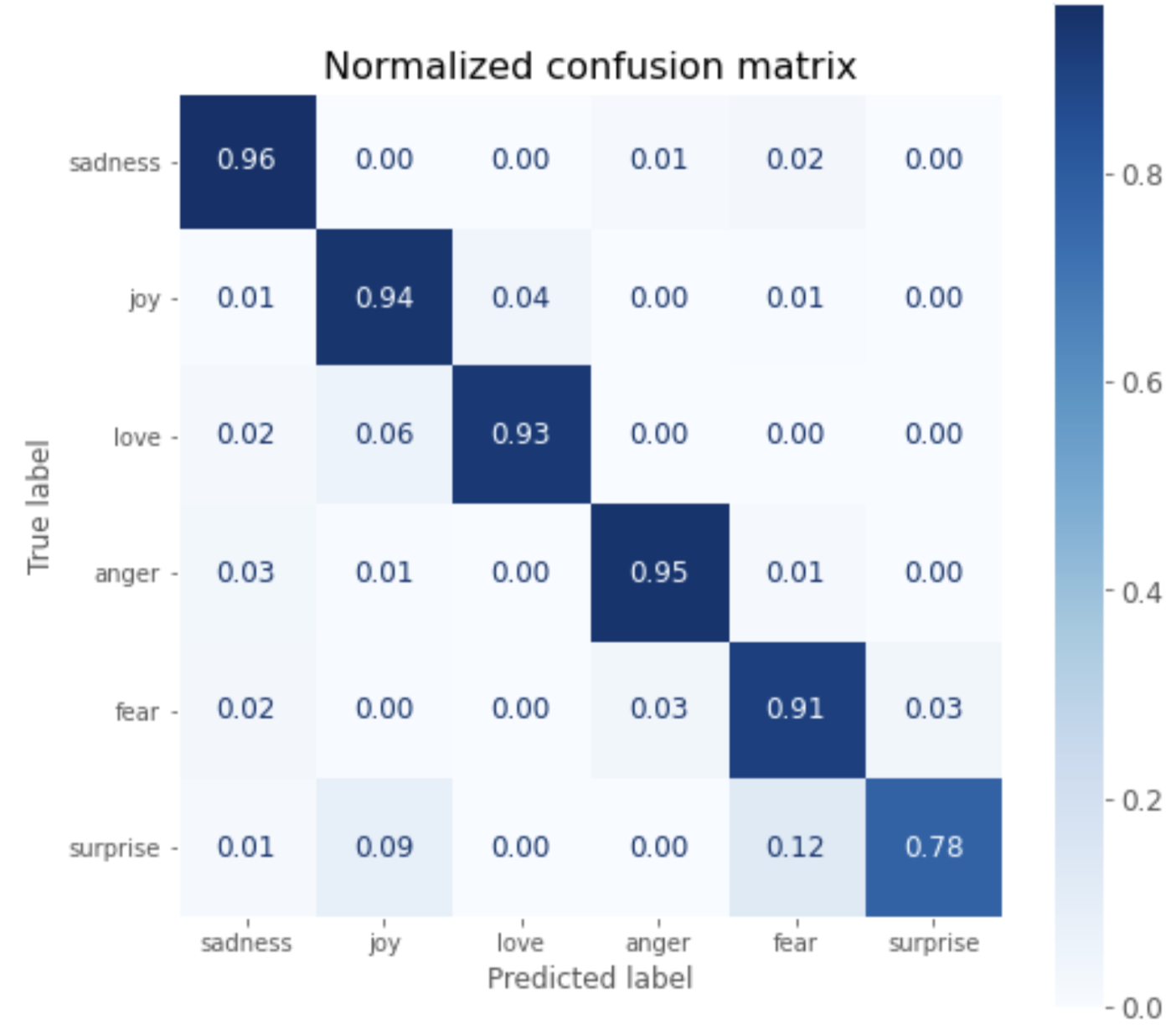
surprise以外は90%以上の正解率となっていることが分かります。

モデルの保存

ラベル情報を設定し、save_model()でモデルを保存します。

id2label = {}
for i in range(dataset["train"].features["label"].num_classes):
    id2label[i] = dataset["train"].features["label"].int2str(i)

label2id = {}
for i in range(dataset["train"].features["label"].num_classes):
    label2id[dataset["train"].features["label"].int2str(i)] = i

trainer.model.config.id2label = id2label
trainer.model.config.label2id = label2id

trainer.save_model(f"./{model_name}")

保存結果は以下のようなディレクトリ構成となります。

sample-distilbert-text-classification
├── config.json
├── pytorch_model.bin
├── special_tokens_map.json
├── tokenizer_config.json
├── training_args.bin
└── vocab.txt

ロードして推論

保存したTokenizerとモデルをPyTorchモデルとしてロードします。

saved_tokenizer = AutoTokenizer.from_pretrained(f"./{model_name}")
saved_model = AutoModelForSequenceClassification.from_pretrained(f"./{model_name}").to(device)

サンプルテキストを推論してみます。

inputs = saved_tokenizer(sample_text, return_tensors="pt")

new_model.eval()

with torch.no_grad():
    outputs = saved_model(
        inputs["input_ids"].to(device),
        inputs["attention_mask"].to(device),
    )

outputs.logits

tensor([[-0.5823,  2.9460, -1.4961,  0.1718, -0.0931, -1.4067]],
       device='cuda:0')

logitsを推論ラベルに変換すると、サンプルテキストの感情はjoyと推論されていることが分かります。

y_preds = np.argmax(outputs.logits.to('cpu').detach().numpy().copy(), axis=1)

def id2label(x):
    return new_model.config.id2label[x]

y_dash = [id2label(x) for x in y_preds]

>> y_dash

['joy']

Google Colaboratory コード

以下にコードのまとめを記載します。

from datasets import load_dataset
from transformers import AutoModelForSequenceClassification, AutoTokenizer
from transformers import TrainingArguments
from transformers import Trainer
from sklearn.metrics import accuracy_score, f1_score
from sklearn.metrics import ConfusionMatrixDisplay, confusion_matrix
import torch
import matplotlib.pyplot as plt
import numpy as np

plt.style.use('ggplot')

# checkpoint
model_ckpt = "distilbert-base-uncased"

# get dataset
dataset = load_dataset("emotion")

# get tokenizer
tokenizer = AutoTokenizer.from_pretrained(model_ckpt)

# get model
device = torch.device("cuda" if torch.cuda.is_available() else "cpu")
num_labels = dataset["train"].features["label"].num_classes
model = (AutoModelForSequenceClassification
    .from_pretrained(model_ckpt, num_labels=num_labels)
    .to(device))

# tokenize
def tokenize(batch):
    return tokenizer(batch["text"], padding=True, truncation=True)
dataset_encoded = dataset.map(tokenize, batched=True, batch_size=None)

# preparation for training
batch_size = 16
logging_steps = len(dataset_encoded["train"]) // batch_size
model_name = f"sample-text-classification-distilbert"
training_args = TrainingArguments(
    output_dir=model_name,
    num_train_epochs=2,
    learning_rate=2e-5,
    per_device_train_batch_size=batch_size,
    per_device_eval_batch_size=batch_size,
    weight_decay=0.01,
    evaluation_strategy="epoch",
    disable_tqdm=False,
    logging_steps=logging_steps,
    push_to_hub=False,
    log_level="error",
)

# define evaluation metrics
def compute_metrics(pred):
    labels = pred.label_ids
    preds = pred.predictions.argmax(-1)
    f1 = f1_score(labels, preds, average="weighted")
    acc = accuracy_score(labels, preds)
    return {"accuracy": acc, "f1": f1}

# train
trainer = Trainer(
    model=model, args=training_args,
    compute_metrics=compute_metrics,
    train_dataset=dataset_encoded["train"],
    eval_dataset=dataset_encoded["validation"],
    tokenizer=tokenizer
)
trainer.train()

# eval
preds_output = trainer.predict(dataset_encoded["validation"])

y_preds = np.argmax(preds_output.predictions, axis=1)
y_valid = np.array(dataset_encoded["validation"]["label"])
labels = dataset_encoded["train"].features["label"].names

def plot_confusion_matrix(y_preds, y_true, labels):
    cm = confusion_matrix(y_true, y_preds, normalize="true")
    fig, ax = plt.subplots(figsize=(8, 8))
    plt.rcParams.update({'font.size': 12})
    disp = ConfusionMatrixDisplay(confusion_matrix=cm, display_labels=labels)
    disp.plot(cmap="Blues", values_format=".2f", ax=ax, colorbar=True)
    plt.grid(None)
    plt.title("Normalized confusion matrix", fontsize=16)
    plt.show()
plot_confusion_matrix(y_preds, y_valid, labels)

# labeling
id2label = {}
for i in range(dataset["train"].features["label"].num_classes):
    id2label[i] = dataset["train"].features["label"].int2str(i)

label2id = {}
for i in range(dataset["train"].features["label"].num_classes):
    label2id[dataset["train"].features["label"].int2str(i)] = i

trainer.model.config.id2label = id2label
trainer.model.config.label2id = label2id


# save
trainer.save_model(f"./{model_name}")

# load
new_tokenizer = AutoTokenizer\
    .from_pretrained(f"./{model_name}")

new_model = (AutoModelForSequenceClassification
    .from_pretrained(f"./{model_name}")
    .to(device))

# infer with sample text
inputs = new_tokenizer(sample_text, return_tensors="pt")
new_model.eval()
with torch.no_grad():
    outputs = new_model(
        inputs["input_ids"].to(device),
        inputs["attention_mask"].to(device),
    )
y_preds = np.argmax(outputs.logits.to('cpu').detach().numpy().copy(), axis=1)
def id2label(x):
    return new_model.config.id2label[x]
y_dash = [id2label(x) for x in y_preds]
y_dash