What is Ridge Regression

Ridge regression, also known as L2 regularization, is a regularization technique used to address the issue of multicollinearity in linear regression models. Multicollinearity arises when predictor variables are highly correlated, leading to unstable and unreliable estimates of the regression coefficients. By incorporating a penalty term in the objective function, ridge regression shrinks the regression coefficients, resulting in a more stable and robust model.

Mathematical Foundation

Cost Function

In linear regression, we aim to find the relationship between the input features (independent variables) and the target variable (dependent variable) by fitting a linear function to the data. The cost function, also known as the objective function or loss function, is used to measure the error between the predicted values and the actual values. The most commonly used cost function in linear regression is the Mean Squared Error (MSE) function:

where:

• m is the number of training examples
• h_\theta(x^{(i)}) is the predicted value for the i-th example
• y^{(i)} is the actual value for the i-th example
• \theta is the parameter vector of the model

Our goal is to minimize the cost function J(\theta), which means finding the optimal values for the parameters \theta that result in the lowest error.

L2 Penalty Term

In Ridge Regression, we add an L2 penalty term to the cost function to penalize large parameter values. This regularization term helps to prevent overfitting by constraining the complexity of the model. The L2 penalty term is defined as:

where:

• \lambda is the regularization parameter (also known as the ridge coefficient), which controls the strength of the regularization
• n is the number of features (excluding the bias term)
• \theta_j is the j-th parameter in the parameter vector \theta

With the L2 penalty term, the cost function for Ridge Regression becomes:

The goal now is to minimize this modified cost function J(\theta) by finding the optimal values for the parameters \theta. As \lambda increases, the penalty term has a stronger effect on the cost function, leading to a higher bias but lower variance model. Conversely, as \lambda decreases, the penalty term has a weaker effect, leading to a lower bias but higher variance model.

Implementing Ridge Regression in Python

In this chapter, I will demonstrate the implementation of ridge regression in Python using the California housing dataset. We will plot the results of linear regression and ridge regression with varying regularization parameters to interpret their effects on the model.

First, let's import the necessary libraries:

import numpy as np
import pandas as pd
import matplotlib.pyplot as plt
import seaborn as sns

from sklearn.datasets import fetch_california_housing
from sklearn.model_selection import train_test_split
from sklearn.preprocessing import StandardScaler
from sklearn.linear_model import LinearRegression, Ridge
from sklearn.metrics import mean_squared_error

Now, we will load the California housing dataset and preprocess it by splitting it into training and testing sets and scaling the features:

# Load the dataset
data = fetch_california_housing()
X, y = data['data'], data['target']

# Split the dataset into training and testing sets
X_train, X_test, y_train, y_test = train_test_split(X, y, test_size=0.2, random_state=42)

# Scale the features
scaler = StandardScaler()
X_train_scaled = scaler.fit_transform(X_train)
X_test_scaled = scaler.transform(X_test)

We will fit both linear regression and ridge regression models with varying regularization parameters to compare their performance:

# Initialize models
linear_regression = LinearRegression()
ridge_regressions = [Ridge(alpha=alpha) for alpha in np.logspace(-3, 3, 7)]

# Fit models
linear_regression.fit(X_train_scaled, y_train)
for ridge_regression in ridge_regressions:
    ridge_regression.fit(X_train_scaled, y_train)

Now, we will evaluate the models using mean squared error (MSE) and create a plot to visualize the results:

# Evaluate models
mse_linear_regression = mean_squared_error(y_test, linear_regression.predict(X_test_scaled))
mse_ridge_regressions = [mean_squared_error(y_test, ridge_regression.predict(X_test_scaled)) for ridge_regression in ridge_regressions]

# Set up the plot
plt.figure(figsize=(10, 6))
sns.set(style="whitegrid")
plt.xscale("log")
plt.xlabel("Regularization Parameter (alpha)")
plt.ylabel("Mean Squared Error")
plt.title("Linear Regression vs Ridge Regression")

# Plot the results
plt.plot(np.logspace(-3, 3, 7), [mse_linear_regression] * 7, label="Linear Regression", linestyle="--", marker="o", color="blue")
plt.plot(np.logspace(-3, 3, 7), mse_ridge_regressions, label="Ridge Regression", linestyle="--", marker="o", color="red")
plt.legend()

# Show the plot
plt.show()

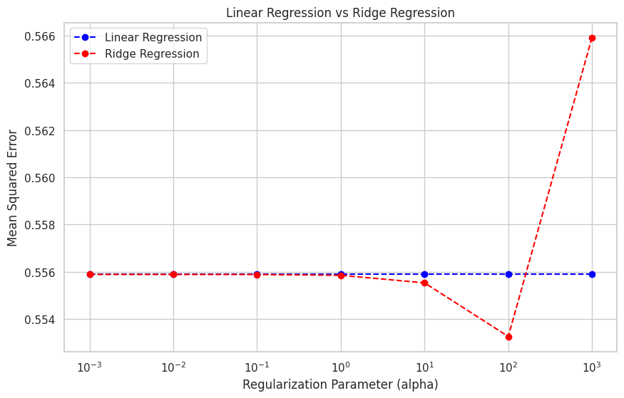
The plot shows the mean squared errors of linear regression and ridge regression models for different regularization parameters. As the regularization parameter (alpha) increases, the ridge regression model's performance improves, initially outperforming the linear regression model. However, as alpha becomes too large, the ridge regression model's performance starts to degrade due to excessive shrinkage of the coefficients.