What is Linear Regression

Linear regression is a machine learning algorithm used to model the relationship between a dependent variable (also known as the response, outcome and objective variable) and one or more independent variables (also known as predictors, features, or input variables). The primary goal of linear regression is to predict the value of the dependent variable based on the values of the independent variables. This is achieved by fitting a linear equation to the observed data points, which can be represented as a straight line in the case of simple linear regression or as a hyperplane for multiple linear regression.

The underlying principle of linear regression is to minimize the difference between the predicted values and the actual values. This difference, known as the residual, is the vertical distance between the data points and the fitted line or hyperplane. By minimizing the sum of the squared residuals, we obtain the best-fitting line or hyperplane that can be used to make predictions about the dependent variable.

Assumptions of Linear Regression

To ensure that the linear regression model provides accurate and reliable predictions, several assumptions must be met:

• Linearity
  There should be a linear relationship between the dependent variable and the independent variables. This can be checked using scatter plots or correlation coefficients.

• Independence
  The independent variables should not be highly correlated with each other. Multicollinearity can lead to unstable estimates and can be addressed by removing redundant variables or using regularization techniques.

• Homoscedasticity
  The variance of the residuals should be constant across all levels of the independent variables. Heteroscedasticity can be detected using scatter plots or diagnostic tests and can be addressed by using weighted least squares or transforming the dependent variable.

• Normality
  The residuals should be normally distributed. This can be checked using histograms, Q-Q plots, or statistical tests such as the Shapiro-Wilk test. Non-normality can be addressed by transforming the dependent variable or using robust regression techniques.

• Independence of Errors
  The residuals should be independent of each other. This can be checked using the Durbin-Watson test or by plotting the residuals against time or the predicted values. Autocorrelation can be addressed by using time series models or incorporating lagged variables.

Simple Linear Regression

In simple linear regression, we aim to establish a linear relationship between a single independent variable (X) and the dependent variable (Y). The equation for this relationship can be written as:

Y = \beta_0 + \beta_1X + \epsilon

where:

• Y is the dependent variable
• X is the independent variable
• \beta_0 is the intercept of the line (the value of Y when X is 0)
• \beta_1 is the slope of the line (the change in Y for a unit change in X)
• \epsilon is the error term (the difference between the actual and predicted values of Y)

The best-fit line is the one that minimizes the sum of squared residuals (the squared differences between the actual and predicted values of Y).

Least Squares Method

The least squares method is a mathematical approach to finding the best-fit line by minimizing the sum of squared residuals. The estimates for the intercept and slope of the best-fit line can be calculated using the following formulas:

\beta_1 = \frac{\sum_{i=1}^n (X_i - \bar{X})(Y_i - \bar{Y})}{\sum_{i=1}^n (X_i - \bar{X})^2}

\beta_0 = \bar{Y} - \beta_1\bar{X}

where:

• n is the number of data points
• X_i and Y_i are the individual data points
• \bar{X} and \bar{Y} are the means of the independent and dependent variables, respectively

Evaluating Model Performance

Once the best-fit line is obtained, we need to evaluate the model's performance to ensure that it is a good fit for the data. Some common metrics used to assess the performance of a simple linear regression model are:

Coefficient of Determination (R^2)

This metric measures the proportion of the variance in the dependent variable that can be explained by the independent variable. An R^2 value close to 1 indicates a strong relationship, while an R^2 value close to 0 indicates a weak relationship.

R^2 = 1 - \frac{\sum_{i=1}^n (Y_i - \hat{Y}i)^2}{\sum{i=1}^n (Y_i - \bar{Y})^2}

where:

• \hat{Y}_i is the predicted value of Y for the i^{th} data point

Mean Squared Error (MSE)

This metric calculates the average squared difference between the actual and predicted values of the dependent variable.

MSE = \frac{1}{n}\sum_{i=1}^n (Y_i - \hat{Y}_i)^2

A lower MSE indicates a better fit of the model to the data.

Multiple Linear Regression

Multiple linear regression extends the concept of simple linear regression to include multiple independent variables. The equation for the relationship between the dependent variable (Y) and the independent variables (X_1, X_2, ..., X_p) can be written as:

Y = \beta_0 + \beta_1X_1 + \beta_2X_2 + \cdots + \beta_pX_p + \epsilon

where:

• Y is the dependent variable
• X_1, X_2, ..., X_p are the independent variables
• \beta_0 is the intercept of the hyperplane
• \beta_1, \beta_2, ..., \beta_p are the coefficients for the independent variables
• \epsilon is the error term (the difference between the actual and predicted values of Y)

Matrix Approach

In multiple linear regression, we use the matrix approach to estimate the coefficients of the independent variables. The least squares estimates can be obtained by solving the following matrix equation:

\boldsymbol{\beta} = (\mathbf{X}^T\mathbf{X})^{-1}\mathbf{X}^T\mathbf{Y}

where:

• \boldsymbol{\beta} is a vector containing the coefficients (\beta_0, \beta_1, ..., \beta_p)
• \mathbf{X} is the matrix of independent variables, with each row representing a data point and each column representing an independent variable
• \mathbf{Y} is the vector of dependent variable values

Handling Multicollinearity

Multicollinearity arises when two or more independent variables are highly correlated. It can lead to unstable estimates and make it difficult to interpret the coefficients of the independent variables. To detect multicollinearity, we can calculate the variance inflation factor (VIF) for each independent variable:

VIF_i = \frac{1}{1 - R_i^2}

where R_i^2 is the R^2 value obtained by regressing the i^{th} independent variable on the other independent variables. A VIF value greater than 10 indicates a high degree of multicollinearity.

To address multicollinearity, we can:

• Remove one of the correlated variables
• Combine correlated variables into a single variable (e.g., by taking their average)
• Apply regularization techniques, such as ridge or lasso regression

Feature Selection and Scaling

In multiple linear regression, it is essential to select the most relevant independent variables to avoid overfitting and improve model interpretability. Feature selection techniques, such as stepwise regression, recursive feature elimination, and LASSO, can be used to identify the most important variables.

Additionally, when the independent variables have different scales, it can be challenging to compare their coefficients. In such cases, feature scaling methods, such as normalization or standardization, can be applied to bring all variables to a similar scale.

Implementing Linear Regression in Python

In this chapter, I will implement both simple and multiple linear regression using Python and the California Housing dataset. This dataset is a popular choice for regression tasks and is available in the scikit-learn library.

First, let's import the necessary libraries and load the California Housing dataset from the scikit-learn library.

import numpy as np
import pandas as pd
import matplotlib.pyplot as plt
import seaborn as sns
from sklearn.datasets import fetch_california_housing
from sklearn.model_selection import train_test_split
from sklearn.linear_model import LinearRegression
from sklearn.metrics import mean_squared_error, r2_score

# Load the California Housing dataset
dataset = fetch_california_housing()
X = pd.DataFrame(dataset.data, columns=dataset.feature_names)
y = dataset.target

# Display the first few rows of the dataset
print(X.head())

	MedInc	HouseAge	AveRooms	AveBedrms	Population	AveOccup	Latitude	Longitude
0	8.3252	41.0	6.984127	1.023810	322.0	2.555556	37.88	-122.23
1	8.3014	21.0	6.238137	0.971880	2401.0	2.109842	37.86	-122.22
2	7.2574	52.0	8.288136	1.073446	496.0	2.802260	37.85	-122.24
3	5.6431	52.0	5.817352	1.073059	558.0	2.547945	37.85	-122.25
4	3.8462	52.0	6.281853	1.081081	565.0	2.181467	37.85	-122.25

Simple Linear Regression

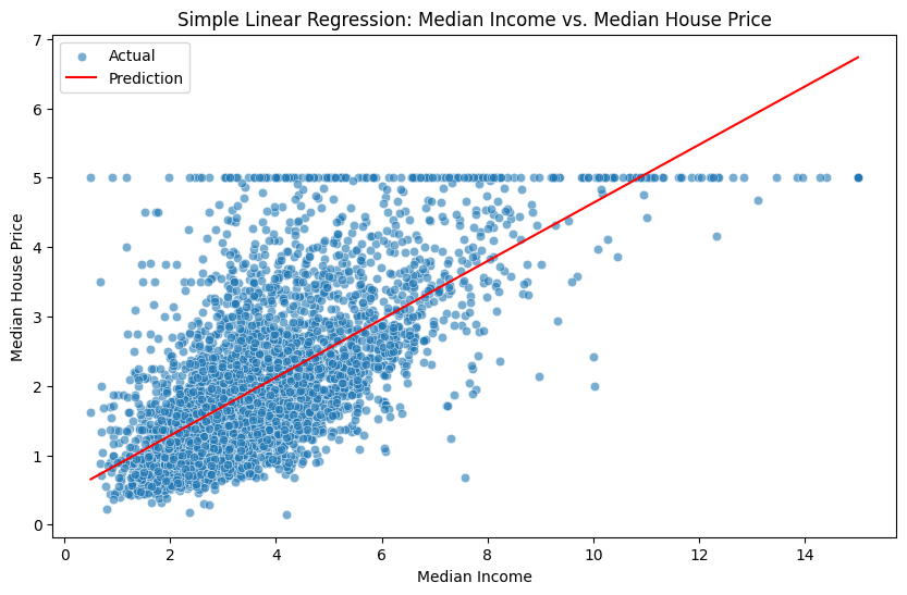
We will start by implementing simple linear regression using the MedInc feature, which represents the median income in a given area, to predict the median house price.

Split the data into training and testing sets.

X_simple = X[["MedInc"]]
X_train_simple, X_test_simple, y_train, y_test = train_test_split(X_simple, y, test_size=0.2, random_state=42)

Create a simple linear regression model and fit it to the training data.

simple_lr = LinearRegression()
simple_lr.fit(X_train_simple, y_train)

Evaluate the model's performance using MSE and R^2 score.

y_pred_simple = simple_lr.predict(X_test_simple)
mse_simple = mean_squared_error(y_test, y_pred_simple)
r2_simple = r2_score(y_test, y_pred_simple)

print("Simple Linear Regression - MSE:", mse_simple)
print("Simple Linear Regression - R² Score:", r2_simple)

Simple Linear Regression - MSE: 0.7091157771765549
Simple Linear Regression - R² Score: 0.45885918903846656

Plot the best-fit line using matplotlib and seaborn.

plt.figure(figsize=(10, 6))
sns.scatterplot(x=X_test_simple["MedInc"], y=y_test, alpha=0.6, label="Actual")
sns.lineplot(x=X_test_simple["MedInc"], y=y_pred_simple, color="red", label="Prediction")
plt.xlabel("Median Income")
plt.ylabel("Median House Price")
plt.title("Simple Linear Regression: Median Income vs. Median House Price")
plt.legend()
plt.show()

Multiple Linear Regression

Now let's implement multiple linear regression using all the features in the dataset.

Split the data into training and testing sets.

X_train, X_test, y_train, y_test = train_test_split(X, y, test_size=0.2, random_state=42)

Create a multiple linear regression model and fit it to the training data.

multiple_lr = LinearRegression()
multiple_lr.fit(X_train, y_train)

Evaluate the model's performance using mean squared error (MSE) and R^2 score.

y_pred_multiple = multiple_lr.predict(X_test)
mse_multiple = mean_squared_error(y_test, y_pred_multiple)
r2_multiple = r2_score(y_test, y_pred_multiple)

print("Multiple Linear Regression - MSE:", mse_multiple)
print("Multiple Linear Regression - R² Score:", r2_multiple)

Multiple Linear Regression - MSE: 0.5558915986952444
Multiple Linear Regression - R² Score: 0.5757877060324508

Now let's compare the performance of the simple and multiple linear regression models using their MSE and R^2 scores.

print("Simple Linear Regression - MSE:", mse_simple)
print("Simple Linear Regression - R² Score:", r2_simple)
print("Multiple Linear Regression - MSE:", mse_multiple)
print("Multiple Linear Regression - R² Score:", r2_multiple)

Simple Linear Regression - MSE: 0.709
Simple Linear Regression - R² Score: 0.459
Multiple Linear Regression - MSE: 0.556
Multiple Linear Regression - R² Score: 0.576

Based on the results, the multiple linear regression model should generally have a lower MSE and a higher R^2 score compared to the simple linear regression model. This indicates that the multiple linear regression model is a better fit for the data and can better predict the median house price using the given features.

References

https://www.spiceworks.com/tech/artificial-intelligence/articles/what-is-linear-regression/
https://www.analyticsvidhya.com/blog/2021/10/everything-you-need-to-know-about-linear-regression/
https://www.spiceworks.com/tech/artificial-intelligence/articles/what-is-linear-regression/
https://www.youtube.com/watch?v=nk2CQITm_eo&ab_channel=StatQuestwithJoshStarmer