What is Lasso Regression

Lasso Regression, also known as Least Absolute Shrinkage and Selection Operator, is a linear regression model that introduces regularization to improve model performance and interpretability. The primary objective of Lasso Regression is to minimize the complexity of the model by adding an L1 penalty term to the cost function, which helps in feature selection and prevents overfitting.

Need for Regularization

In machine learning, overfitting occurs when a model learns the noise in the training data and performs poorly on unseen data. Regularization is a technique used to address this issue by adding a penalty term to the cost function. By doing so, the model is forced to focus on the most relevant features and avoid fitting the noise.

Regularization methods can be broadly classified into two categories: L1 regularization and L2 regularization. Lasso Regression uses L1 regularization, which results in a sparse model by setting some coefficients to zero. This property of Lasso Regression makes it an ideal candidate for feature selection, especially when dealing with a large number of features.

Mathematical Foundations of Lasso Regression

Cost Function

In linear regression, the cost function, also known as the objective function, is used to measure the difference between the predicted values and the actual values. The goal is to minimize this cost function to obtain the optimal coefficients for the model. The cost function for linear regression is given by the Mean Squared Error (MSE):

J(\boldsymbol{\beta}) = \frac{1}{n}\sum_{i=1}^n (y_i - \boldsymbol{x}_i^T \boldsymbol{\beta})^2

Where n is the number of observations, y_i represents the actual output, \boldsymbol{x}_i^T is the transpose of the i^{th} input vector, and \boldsymbol{\beta} is the vector of coefficients.

L1 Penalty Term

In Lasso Regression, an L1 penalty term is added to the cost function to introduce regularization. The L1 penalty term is given by:

L1(\boldsymbol{\beta}) = \lambda \sum_{j=1}^p |\beta_j|

Where \lambda is the regularization parameter, p is the number of features, and \beta_j is the j^{th} coefficient. The L1 penalty term encourages sparsity by forcing some of the coefficients to be exactly zero.

Lagrange Multiplier

By incorporating the L1 penalty term into the cost function, we obtain the Lasso Regression objective function:

J(\boldsymbol{\beta}) = \frac{1}{n}\sum_{i=1}^n (y_i - \boldsymbol{x}i^T \boldsymbol{\beta})^2 + \lambda \sum{j=1}^p |\beta_j|

The Lagrange multiplier, \lambda, controls the trade-off between fitting the data and enforcing sparsity in the model. A higher value of \lambda results in a more sparse model, while a lower value of \lambda allows the model to fit the data more closely.

Solution Paths and the Lasso Constraint

A key aspect of Lasso Regression is the solution path, which illustrates how the coefficient estimates change as a function of the regularization parameter, \lambda. As \lambda increases, more coefficients are forced to zero, and the model becomes sparser.

The Lasso constraint can be represented geometrically by an L1 norm ball centered at the origin, with a radius proportional to \frac{1}{\lambda}. The Lasso Regression solution corresponds to the first point where the contour of the cost function intersects the L1 norm ball. Due to the geometry of the L1 norm ball, the solution is more likely to lie on the axes, resulting in sparse models with some coefficients exactly equal to zero.

Implementation of Lasso Regression in Python

In this chapter, I will implement Lasso Regression using the California Housing dataset and visualize the transition of coefficients as the regularization parameter increases.

import numpy as np
import pandas as pd
import matplotlib.pyplot as plt
import seaborn as sns
from sklearn.datasets import fetch_california_housing
from sklearn.linear_model import Lasso
from sklearn.model_selection import train_test_split
from sklearn.preprocessing import StandardScaler

# Load the California Housing dataset
data = fetch_california_housing()
X = data['data']
y = data['target']
feature_names = data['feature_names']

# Split the dataset into train and test sets
X_train, X_test, y_train, y_test = train_test_split(X, y, test_size=0.3, random_state=42)

# Standardize the data
scaler = StandardScaler()
X_train_scaled = scaler.fit_transform(X_train)
X_test_scaled = scaler.transform(X_test)

# Set the range of regularization parameter values
lambdas = np.logspace(-4, 1, 100)

# Store the coefficients for each lambda value
coefficients = []

# Fit Lasso Regression for each lambda value and store the coefficients
for lmbda in lambdas:
    lasso = Lasso(alpha=lmbda, max_iter=10000)
    lasso.fit(X_train_scaled, y_train)
    coefficients.append(lasso.coef_)

# Plot the transition of coefficients using Matplotlib and Seaborn
plt.figure(figsize=(12, 8))
sns.set(style='whitegrid', palette='muted')

# Customize plot appearance
for i, feature in enumerate(feature_names):
    sns.lineplot(x=lambdas, y=np.array(coefficients)[:, i], label=feature)

plt.xscale('log')
plt.xlabel('Regularization Parameter (λ)', fontsize=14)
plt.ylabel('Coefficient Values', fontsize=14)
plt.title('Transition of Coefficients in Lasso Regression', fontsize=16, fontweight='bold')
plt.legend(fontsize=12, loc='upper right')

# Display the plot
plt.show()

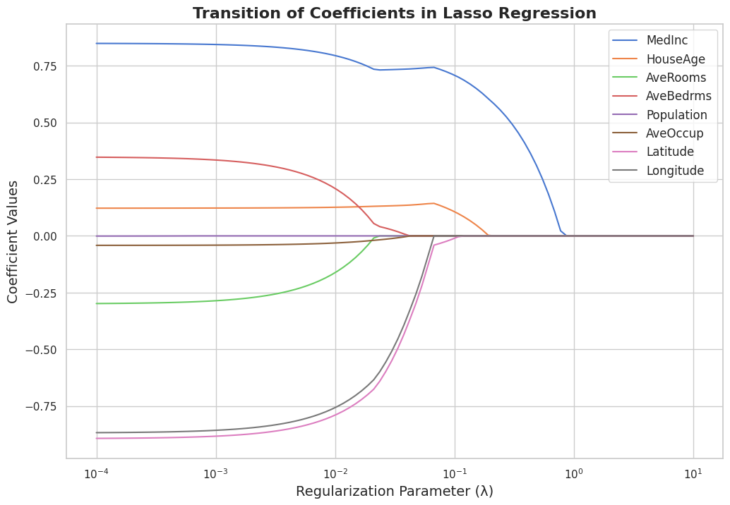
This script loads the California Housing dataset, splits it into train and test sets, and standardizes the features. Then, it fits a Lasso Regression model for a range of regularization parameter values (\lambda) and stores the coefficients.

Finally, it uses Matplotlib and Seaborn to create a visually appealing plot displaying the transition of coefficients as the regularization parameter increases. The plot demonstrates the effect of Lasso Regression on the coefficients, showing how they shrink and some become exactly zero as \lambda increases. This is the essence of Lasso Regression's ability to promote sparsity and perform feature selection.