What is K-Nearest Neighbors (KNN) Regression

K-Nearest Neighbors (KNN) Regression is a non-parametric supervised learning algorithm used for predicting continuous target variables. Unlike parametric models, KNN Regression doesn't make any assumptions about the underlying data distribution or the relationship between variables. Instead, it estimates the target variable by taking the average of observations in the nearby vicinity, where the proximity is measured by a distance metric. KNN Regression is a simple yet powerful algorithm that can model complex, non-linear relationships.

Choosing the Right 'K'

The choice of 'K' is a crucial factor that influences the performance of the KNN algorithm. A smaller value for 'K' can lead to a more complex model that captures the local patterns in the data, but it may be sensitive to noise, leading to overfitting. On the other hand, a larger value for 'K' can lead to a more generalized model that is less sensitive to noise, but it may overlook important local patterns, resulting in underfitting. Choosing the right value of 'K' can be achieved through cross validation and experimentation.

Comparison to Linear Regression

Here are key differences between linear regression and KNN regression.

• Model Assumptions
  Linear regression assumes that there is a linear relationship between the independent and dependent variables, and it tries to find the best-fitting straight line through the data points. KNN Regression, on the other hand, is a non-parametric method, which means it doesn't make any assumptions about the underlying data distribution or the relationship between variables. This makes KNN regression more flexible and capable of modeling complex, non-linear relationships.

• Model Complexity
  Linear regression results in a simple, interpretable model represented by a straight line (or a hyperplane in the case of multiple independent variables). KNN regression can produce more complex models depending on the choice of 'K' and the distance metric used. While this flexibility can be advantageous in certain situations, it can also make the model more prone to overfitting, especially with small 'K' values.

• Feature Scaling
  Linear regression is less sensitive to the scale of the features, as it estimates the coefficients for each feature independently. However, KNN regression relies on distance metrics to find the nearest neighbors, which makes it sensitive to the scale of the features. Consequently, feature scaling (e.g., normalization or standardization) is an essential preprocessing step in KNN Regression.

• Training and Prediction Time
  Linear regression has a closed-form solution that can be computed efficiently, making the training process relatively fast. Once the coefficients are estimated, predictions can be made quickly as well. In contrast, KNN regression doesn't have an explicit training phase, as it stores the entire training dataset to make predictions. As a result, the prediction time for KNN regression can be significantly slower, particularly for large datasets.

• Handling of Outliers
  Linear regression is sensitive to outliers in the data, as they can have a significant impact on the estimated coefficients and, consequently, the model's performance. KNN regression, with an appropriate choice of 'K,' is generally more robust to outliers, as it takes into account multiple neighboring points when making predictions.

Implementing KNN Regression with Python

In this chapter, I will demonstrate how to implement KNN regression in Python using the California Housing dataset. We will also explore the effect of varying the value of 'K' and choose the best 'K' through cross validation.

First, let's import the required libraries:

import numpy as np
import pandas as pd
import matplotlib.pyplot as plt
import seaborn as sns
from sklearn import datasets
from sklearn.model_selection import train_test_split, GridSearchCV
from sklearn.preprocessing import StandardScaler
from sklearn.neighbors import KNeighborsRegressor
from sklearn.metrics import mean_squared_error

Now, let's load the California Housing dataset and perform basic preprocessing:

# Load the California Housing dataset
california_housing = datasets.fetch_california_housing()
X = california_housing.data
y = california_housing.target

# Split the dataset into training and testing sets
X_train, X_test, y_train, y_test = train_test_split(X, y, test_size=0.2, random_state=42)

# Scale the features
scaler = StandardScaler()
X_train_scaled = scaler.fit_transform(X_train)
X_test_scaled = scaler.transform(X_test)

Next, we will implement the KNN regression model and evaluate its performance using cross validation:

# Initialize a range of K values
k_values = np.arange(1, 31)

# Perform GridSearchCV to find the best K value
knn_regressor = KNeighborsRegressor()
param_grid = {'n_neighbors': k_values}
grid_search = GridSearchCV(knn_regressor, param_grid, cv=5, scoring='neg_mean_squared_error', n_jobs=-1)
grid_search.fit(X_train_scaled, y_train)

# Obtain the best K value and corresponding performance
best_k = grid_search.best_params_['n_neighbors']
best_performance = -grid_search.best_score_
print(f"Best K value: {best_k}")
print(f"Best performance (Mean Squared Error): {best_performance}")

Now, let's create a cool and informative plot showing the KNN regression performance with various K values:

# Retrieve the performance for each K value
performance = -grid_search.cv_results_['mean_test_score']

# Set up the plotting environment
sns.set(style="darkgrid")
plt.figure(figsize=(10, 6))

# Plot the performance for each K value
plt.plot(k_values, performance, marker='o', linestyle='-', linewidth=2)
plt.xlabel("Number of Neighbors (K)")
plt.ylabel("Mean Squared Error")
plt.title("KNN Regression Performance with Various K")

# Highlight the best K value
plt.scatter(best_k, best_performance, s=200, c='red', marker='x', zorder=5)
plt.annotate(f"Best K: {best_k}",
             xy=(best_k, best_performance),
             xytext=(best_k + 2, best_performance),
             arrowprops=dict(facecolor='black', arrowstyle='->'))

plt.show()

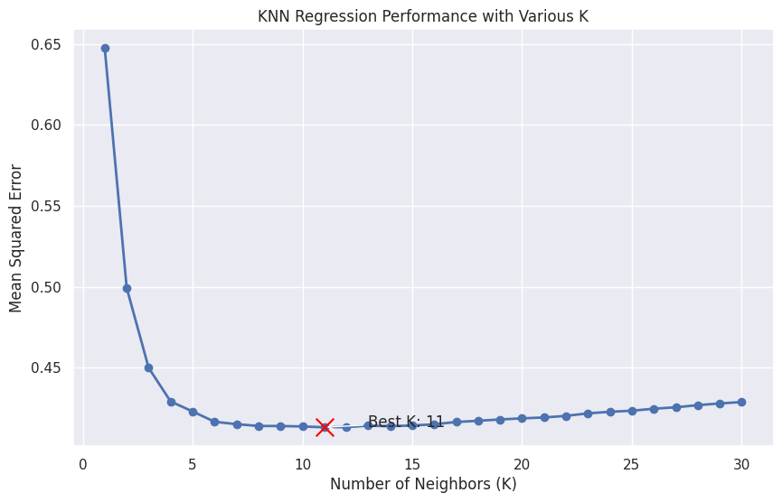
This plot shows the performance of KNN Regression for different values of K, with the best K value highlighted in red. The graph should help you visualize the trade-off between overfitting and underfitting as K varies, making it easier to choose the optimal value for your model.

To plot the KNN regression predictions with various K values, we'll first choose one feature from the California Housing dataset for visualization purposes. We'll use the 'MedInc' (Median Income) feature, which is the first column in the dataset. Then, we'll create a scatterplot of the actual target values and overlay the KNN regression predictions for different K values.

# Extract the 'MedInc' feature for visualization
X_medinc = X_train_scaled[:, 0].reshape(-1, 1)

# Generate a range of 'MedInc' values for plotting
medinc_range = np.linspace(X_medinc.min(), X_medinc.max(), 100).reshape(-1, 1)

# Set up the plotting environment
sns.set(style="darkgrid")
plt.figure(figsize=(12, 8))

# Create a scatterplot of the actual target values
plt.scatter(X_medinc, y_train, s=15, c='gray', label='Actual Data')

# Overlay the KNN Regression predictions for various K values
k_values_to_plot = [1, 5, 10, 20, best_k]
colors = ['red', 'blue', 'green', 'purple', 'orange']
for k, color in zip(k_values_to_plot, colors):
    knn_regressor = KNeighborsRegressor(n_neighbors=k)
    knn_regressor.fit(X_medinc, y_train)
    predictions = knn_regressor.predict(medinc_range)
    plt.plot(medinc_range, predictions, linestyle='-', color=color, label=f'K={k}')

# Customize the plot appearance
plt.xlabel("Median Income (Normalized)")
plt.ylabel("Median House Value")
plt.title("KNN Regression with Various K")
plt.legend()
plt.show()

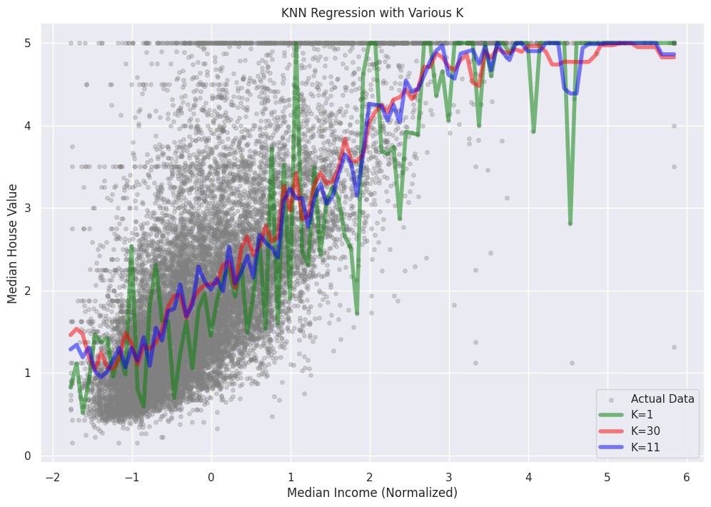
In this plot, we can see how the KNN Regression predictions change for different K values. As K increases, the model becomes smoother and less sensitive to individual data points, reducing the risk of overfitting. However, it's important to choose an appropriate K value to strike a balance between capturing the underlying patterns in the data and avoiding overfitting or underfitting.

References

https://bookdown.org/tpinto_home/Regression-and-Classification/k-nearest-neighbours-regression.html
https://www.youtube.com/watch?v=HVXime0nQeI&ab_channel=StatQuestwithJoshStarmer