
What is Regularization
Regularization is a technique used in machine learning and statistical modeling to reduce the complexity of a model by adding a penalty term to the loss function. This penalty term discourages overfitting and ensures that the model generalizes well on unseen data. In other words, regularization helps in striking a balance between underfitting and overfitting by constraining the model's capacity to learn complex patterns in the data.
Importance of Regularization in Machine Learning
Regularization plays a significant role in machine learning for several reasons:
-
Preventing Overfitting
Overfitting occurs when a model learns the noise in the training data, resulting in poor performance on unseen data. Regularization helps prevent overfitting by penalizing complex models and encouraging simpler ones. -
Feature Selection
Some regularization techniques, such as L1 regularization, can promote sparsity in the model by shrinking some coefficients to zero. This effectively performs feature selection, making the model more interpretable and robust. -
Stability
Regularization techniques, such as L2 regularization, can improve the stability of a model by reducing the sensitivity of the model's coefficients to small changes in the input data. -
Reducing Model Complexity
Regularization constrains the model's capacity, leading to simpler models that are easier to interpret and maintain.
Overfitting and Underfitting
In machine learning, the ultimate goal is to build models that generalize well to unseen data. However, two common challenges arise during the model-building process: overfitting and underfitting. Both can negatively impact a model's performance on new data.
-
Overfitting
Overfitting occurs when a model learns the noise or random fluctuations in the training data instead of the underlying patterns. As a result, the model performs exceptionally well on the training data but poorly on unseen data. Overfitting typically arises when the model is too complex and has a high variance. -
Underfitting
Underfitting occurs when a model is too simple to capture the underlying patterns in the data. Consequently, the model performs poorly on both the training data and unseen data. Underfitting is a result of high bias in the model.
L1 Regularization (Lasso)
L1 regularization, also known as Lasso (Least Absolute Shrinkage and Selection Operator), is a regularization technique that adds the absolute value of the model's coefficients to the loss function. The modified loss function for L1 regularization can be represented as:
where
L1 regularization encourages sparsity in the model by shrinking some coefficients to zero, effectively performing feature selection. This results in a more interpretable and less complex model.
Advantages
-
Feature Selection
L1 regularization can perform feature selection, making the model more interpretable and robust. -
Model Simplicity
By encouraging sparsity in the model's coefficients, L1 regularization leads to simpler models that are easier to interpret and maintain.
Disadvantages
-
Instability
L1 regularization can lead to unstable solutions when there is high multicollinearity between features, as it tends to select only one feature from a group of correlated features. -
Inappropriate for Small Datasets
L1 regularization might not perform well on small datasets, as it can introduce additional bias due to its sparse nature.
L2 Regularization (Ridge)
L2 regularization, also known as Ridge, is another popular regularization technique that adds the square of the model's coefficients to the loss function. The modified loss function for L2 regularization can be represented as:
where
L2 regularization encourages the model to use all features, but with smaller coefficients, reducing overfitting and promoting stability.
Advantages
-
Stability
L2 regularization is more stable than L1 regularization and works well when there is multicollinearity between features, as it distributes the effect of correlated features among them. -
Less Bias
L2 regularization tends to introduce less bias in the model compared to L1 regularization, making it more suitable for smaller datasets.
Disadvantages
-
No Feature Selection
Unlike L1 regularization, L2 regularization does not promote sparsity in the model's coefficients, and therefore, it does not perform feature selection. -
Less Interpretable Models
Since L2 regularization does not encourage sparsity, the resulting models can be less interpretable compared to those obtained using L1 regularization.
Elastic Net Regularization
Elastic Net regularization is a hybrid technique that combines the benefits of both L1 and L2 regularization. It incorporates both the absolute value and the square of the model's coefficients in the loss function. The modified loss function for Elastic Net regularization can be represented as:
where
Elastic Net regularization balances the sparsity-inducing properties of L1 regularization with the stability-promoting properties of L2 regularization.
Advantages
-
Balances L1 and L2 Regularization
Elastic Net regularization balances the sparsity-inducing properties of L1 regularization with the stability-promoting properties of L2 regularization, making it a suitable choice for various problems. -
Feature Selection
Elastic Net regularization can perform feature selection while maintaining the stability of the model, unlike L1 regularization, which can be unstable in the presence of multicollinearity.
Disadvantages
-
Computational Complexity
Elastic Net regularization requires more computational resources compared to L1 or L2 regularization, as it involves optimizing two regularization parameters. -
Hyperparameter Tuning
The additional hyperparameter, l1_ratio, needs to be tuned, which can increase the complexity of the model selection process.
Choosing the Right Regularization Technique
Selecting the appropriate regularization technique depends on various factors, such as the size of the dataset, the presence of multicollinearity, and the desired model properties. Here are some guidelines to help you choose the right regularization method:
-
Dataset Size
For small datasets, L2 regularization is generally more suitable, as it introduces less bias compared to L1 regularization. However, for larger datasets, L1 regularization can be beneficial due to its sparsity-inducing properties, which lead to more interpretable models. -
Multicollinearity
If your dataset has multicollinearity between features, L2 or Elastic Net regularization can be more appropriate, as they distribute the effect of correlated features among them and promote stability. L1 regularization might not work well in such cases, as it tends to select only one feature from a group of correlated features. -
Feature Selection
If you desire a model that performs feature selection, L1 or Elastic Net regularization can be suitable choices, as they encourage sparsity in the model's coefficients. L2 regularization does not perform feature selection, as it does not promote sparsity. -
Model Interpretability
If you prioritize model interpretability, L1 regularization can be a good option due to its sparsity-inducing properties. However, Elastic Net regularization can also lead to interpretable models while maintaining stability in the presence of multicollinearity.
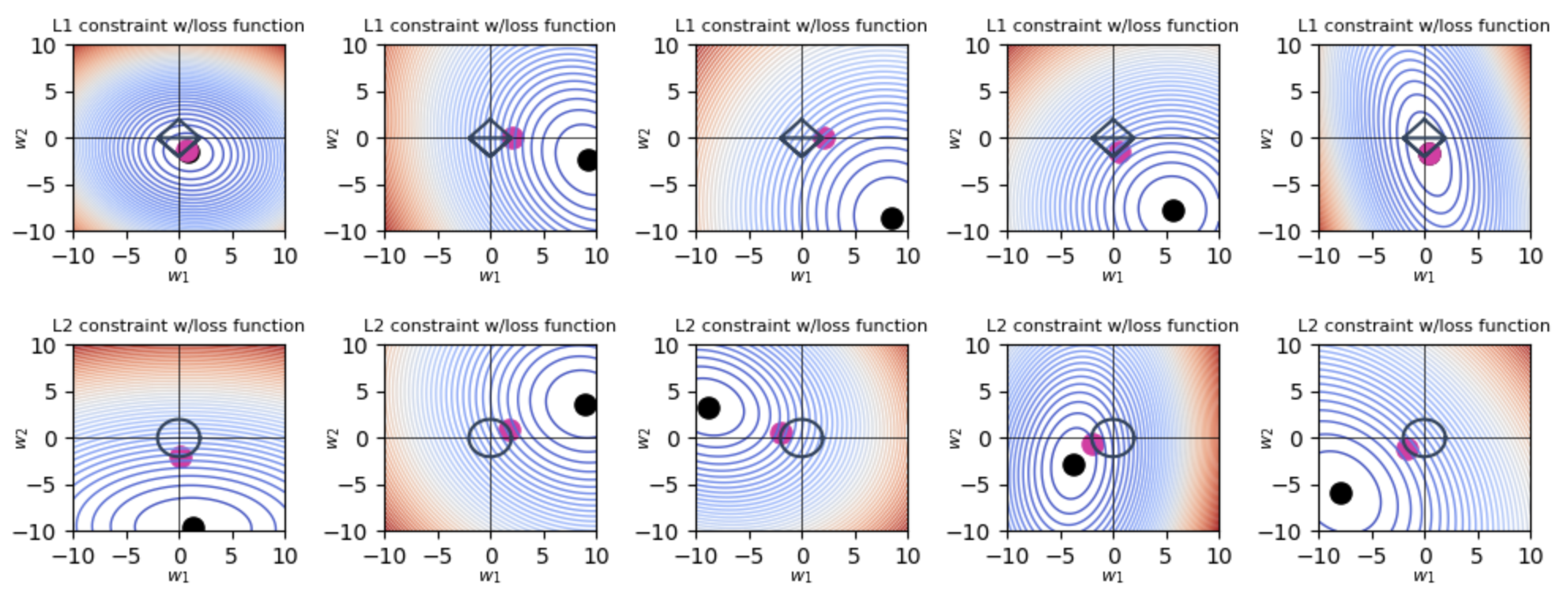
Visualizing L1 and L2 Regularization
Here are scripts for plotting the L1 and L2 regularizations with Python.
2D Plotting
import numpy as np
import matplotlib.pyplot as plt
import glob
import os
import warnings

lmbda = 2
w,h = 10,10

beta0 = np.linspace(-w, w, 100)
beta1 = np.linspace(-h, h, 100)
B0, B1 = np.meshgrid(beta0, beta1)

def diamond(lmbda=1, n=100):
    "get points along diamond at distance lmbda from origin"
    points = []
    x = np.linspace(0, lmbda, num=n // 4)
    points.extend(list(zip(x, -x + lmbda)))
    x = np.linspace(0, lmbda, num=n // 4)
    points.extend(list(zip(x,  x - lmbda)))
    x = np.linspace(-lmbda, 0, num=n // 4)
    points.extend(list(zip(x, -x - lmbda)))
    x = np.linspace(-lmbda, 0, num=n // 4)
    points.extend(list(zip(x,  x + lmbda)))
    return np.array(points)

def circle(lmbda=1, n=100):
    points = []
    for angle in np.linspace(0,np.pi/2, num=n//4):
        x = np.cos(angle) * lmbda
        y = np.sin(angle) * lmbda
        points.append((x,y))
    for angle in np.linspace(np.pi/2,np.pi, num=n//4):
        x = np.cos(angle) * lmbda
        y = np.sin(angle) * lmbda
        points.append((x,y))
    for angle in np.linspace(np.pi, np.pi*3/2, num=n//4):
        x = np.cos(angle) * lmbda
        y = np.sin(angle) * lmbda
        points.append((x,y))
    for angle in np.linspace(np.pi*3/2, 2*np.pi,num=n//4):
        x = np.cos(angle) * lmbda
        y = np.sin(angle) * lmbda
        points.append((x,y))
    return np.array(points)

def loss(b0, b1,
         a = 1,
         b = 1,
         c = 0,
         cx = -10,
         cy = 5):
    return a * (b0 - cx) ** 2 + b * (b1 - cy) ** 2 + c * (b0 - cx) * (b1 - cy)

def select_parameters(lmbda, reg, force_symmetric_loss, force_one_nonpredictive):
    while True:
        a = np.random.random() * 10
        b = np.random.random() * 10
        c = np.random.random() * 4 - 1.5
        if force_symmetric_loss:
            b = a
            c = 0
        elif force_one_nonpredictive:
            if np.random.random() > 0.5:
                a = np.random.random() * 15 - 5
                b = .1
            else:
                b = np.random.random() * 15 - 5
                a = .1
            c = 0
        x, y = 0, 0

        if reg=='L1':
            while np.abs(x) + np.abs(y) <= lmbda:
                x = np.random.random() * 2 * w - w
                y = np.random.random() * 2 * h - h
        else:
            while np.sqrt(x**2 + y**2) <= lmbda:
                x = np.random.random() * 2 * w - w
                y = np.random.random() * 2 * h - h

        Z = loss(B0, B1, a=a, b=b, c=c, cx=x, cy=y)
        loss_at_min = loss(x, y, a=a, b=b, c=c, cx=x, cy=y)
        if (Z >= loss_at_min).all():
            break
    return Z, a, b, c, x, y

def plot_loss(boundary, reg,
              boundary_color='#2D435D',
              boundary_dot_color='#E32CA6',
              force_symmetric_loss=False, force_one_nonpredictive=False,
              show_contours=True, contour_levels=50, show_loss_eqn=False,
              show_min_loss=True,idx=None,fig=None,ax=None,num_trials=None):
    Z, a, b, c, x, y = select_parameters(lmbda, reg,
                          force_symmetric_loss=force_symmetric_loss,
                          force_one_nonpredictive=force_one_nonpredictive)
    eqn = f"{a:.2f}(b0 - {x:.2f})^2 + {b:.2f}(b1 - {y:.2f})^2 + {c:.2f} b0 b1"
    n_col = 5
    if show_loss_eqn:
        ax[idx//n_col, idx%n_col].set_title(eqn, fontsize=10)
    ax[idx//n_col, idx%n_col].set_xlabel("x", fontsize=8, labelpad=0)
    ax[idx//n_col, idx%n_col].set_ylabel("y", fontsize=8, labelpad=-10)
    ax[idx//n_col, idx%n_col].set_xticks([-10,-5,0,5,10])
    ax[idx//n_col, idx%n_col].set_yticks([-10,-5,0,5,10])
    ax[idx//n_col, idx%n_col].set_xlabel(r"$w_1$", fontsize=8)
    ax[idx//n_col, idx%n_col].set_ylabel(r"$w_2$", fontsize=8)
    shape = ""
    if force_symmetric_loss:
        shape = "symmetric "
    elif force_one_nonpredictive:
        shape = "orthogonal "
    ax[idx//n_col, idx%n_col].set_title(f"{reg} constraint w/{shape}loss function", fontsize=8)
    if show_contours:
        ax[idx//n_col, idx%n_col].contour(B0, B1, Z, levels=contour_levels, linewidths=1.0, cmap='coolwarm')
    else:
        ax[idx//n_col, idx%n_col].contourf(B0, B1, Z, levels=contour_levels, cmap='coolwarm')

    ax[idx//n_col, idx%n_col].plot([-w,+w],[0,0], '-', c='k', lw=.5)
    ax[idx//n_col, idx%n_col].plot([0, 0],[-h,h], '-', c='k', lw=.5)

    if boundary is not None:
        ax[idx//n_col, idx%n_col].plot(boundary[:,0], boundary[:,1], '-', lw=1.5, c=boundary_color)

    if show_min_loss:
        ax[idx//n_col, idx%n_col].scatter([x],[y], s=90, c='k')

    eqn = f"{a:.2f}(b0 - {x:.2f})^2 + {b:.2f}(b1 - {y:.2f})^2 + {c:.2f} (b0-{x:.2f}) (b1-{y:.2f})"
    if boundary is not None:
        losses = [loss(*edgeloc, a=a, b=b, c=c, cx=x, cy=y) for edgeloc in boundary]
        minloss_idx = np.argmin(losses)
        coeff = boundary[minloss_idx]
        ax[idx//n_col, idx%n_col].scatter([coeff[0]], [coeff[1]], s=90, c=boundary_dot_color)
        if force_symmetric_loss:
            if reg=='L2':
                ax[idx//n_col, idx%n_col].plot([x,0],[y,0], ':', c='k')
            else:
                ax[idx//n_col, idx%n_col].plot([x,coeff[0]],[y,coeff[1]], ':', c='k')

def plot_2d(reg, force_symmetric_loss=False, force_one_nonpredictive=False,num_trials=None):
    if num_trials <=5:
        fig,ax = plt.subplots(1,5,figsize=(10,2),squeeze=False)
    elif num_trials > 5 and num_trials<=10:
        fig,ax = plt.subplots(2,5,figsize=(10,4))
    elif num_trials > 10 and num_trials<=15:
        fig,ax = plt.subplots(3,5,figsize=(10,6))
        fig.subplots_adjust(hspace=0.6, wspace=0.4)
    if reg == 'L1':
        boundary = diamond(lmbda=lmbda, n=100)
    else:
        boundary = circle(lmbda=lmbda, n=100)
    for i in range(num_trials):
        plot_loss(boundary=boundary, reg=reg,
                  force_symmetric_loss=force_symmetric_loss,
                  force_one_nonpredictive=force_one_nonpredictive,
                  contour_levels=contour_levels,idx=i,fig=fig,ax=ax,num_trials=num_trials)
        shape_fname = ""
        if force_symmetric_loss:
            shape_fname = "symmetric-"
        elif force_one_nonpredictive:
            shape_fname = "orthogonal-"
        plt.tight_layout()

    if num_trials%5!=0:
        k = 5*(1 + num_trials//5)-num_trials
        for i in range(k):
            fig.delaxes(ax[num_trials//5][-i-1])
    plt.show()

n_trials = 5
contour_levels=50
s = 0
np.random.seed(s)
for mode in ["L1", "L2"]:
    plot_2d(reg=mode,num_trials=n_trials)
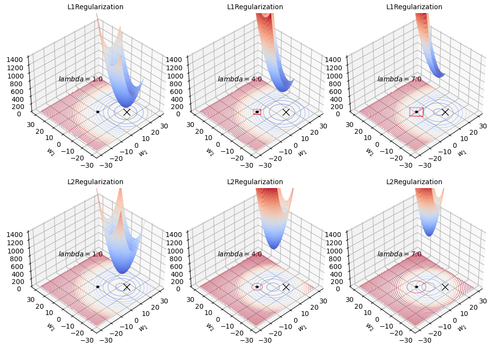
3D Plotting
# https://github.com/parrt/website-explained.ai/blob/master/regularization/code/l2loss_with_penalty.py

import numpy as np
from matplotlib import pyplot as plt
from matplotlib import animation
from mpl_toolkits.mplot3d import Axes3D
from matplotlib import cm
from matplotlib.patches import Circle
import mpl_toolkits.mplot3d.art3d as art3d
import glob
import os
from PIL import Image as PIL_Image

def diamond(lmbda=1, n=100):
    "get points along diamond at distance lmbda from origin"
    points = []
    x = np.linspace(0, lmbda, num=n // 4)
    points.extend(list(zip(x, -x + lmbda)))
    x = np.linspace(0, lmbda, num=n // 4)
    points.extend(list(zip(x,  x - lmbda)))
    x = np.linspace(-lmbda, 0, num=n // 4)
    points.extend(list(zip(x, -x - lmbda)))
    x = np.linspace(-lmbda, 0, num=n // 4)
    points.extend(list(zip(x,  x + lmbda)))
    return np.array(points)

def circle(lmbda=1, n=100):
    points = []
    for angle in np.linspace(0,np.pi/2, num=n//4):
        x = np.cos(angle) * lmbda
        y = np.sin(angle) * lmbda
        points.append((x,y))
    for angle in np.linspace(np.pi/2,np.pi, num=n//4):
        x = np.cos(angle) * lmbda
        y = np.sin(angle) * lmbda
        points.append((x,y))
    for angle in np.linspace(np.pi, np.pi*3/2, num=n//4):
        x = np.cos(angle) * lmbda
        y = np.sin(angle) * lmbda
        points.append((x,y))
    for angle in np.linspace(np.pi*3/2, 2*np.pi,num=n//4):
        x = np.cos(angle) * lmbda
        y = np.sin(angle) * lmbda
        points.append((x,y))
    return np.array(points)

def loss(b0, b1,
         a = 1,
         b = 1,
         c = 0,     # axis stretch
         cx = -10,  # shift center x location
         cy = 5,    # shift center y
         lmbda=1.0,
         yintercept=100):
    eqn = f"{a:.2f}(b0 - {cx:.2f})^2 + {b:.2f}(b1 - {cy:.2f})^2 + {c:.2f} (b0-{cx:.2f}) (b1-{cy:.2f}) + {yintercept}"
    return lmbda * (a * (b0 - cx) ** 2 + b * (b1 - cy) ** 2) + c * (b0 - cx) * (b1 - cy) + yintercept

def loss_l1(b0,b1,a=1,b=1,c=0,cx=-10,cy=5,lmbda=1.0,yintercept=100):
    return lmbda*(a*np.abs(b0-cx) + b*np.abs(b1-cy))

def plot_3d(mode, last_lmbda, stepsize, lmbdas):
    fig = plt.figure(figsize=(10,10))
    plt.subplots_adjust(wspace=0.4, hspace=2.0)
    for i,lmbda in enumerate(lmbdas):
        ax = fig.add_subplot(3,3,i+1, projection='3d')
        ax.set_xlabel("$w_1$", labelpad=0)
        ax.set_ylabel("$w_2$", labelpad=0)
        ax.set_title(mode + "Regularization",fontsize=10)
        ax.tick_params(axis='x', pad=0)
        ax.tick_params(axis='y', pad=0)
        ax.set_zlim(0, 1400)

        cx = 15
        cy = -15

        ax.plot([cx], [cy], marker='x', markersize=10, color='black')
        ax.text(-20,20,800, f"$lambda={lmbda:.1f}$", fontsize=10)

        beta0 = np.linspace(-30, 30, 300)
        beta1 = np.linspace(-30, 30, 300)

        B0, B1 = np.meshgrid(beta0, beta1)

        if mode=='L2':
            Z1 = loss(B0, B1, a=1, b=1, c=0, cx=0, cy=0, lmbda=lmbda, yintercept=0)
            Z2 = loss(B0, B1, a=5, b=5, c=0, cx=cx, cy=cy, yintercept=0)
            Z = Z1 + Z2

        elif mode=='L1':
            Z1 = loss_l1(B0,B1,a=5,b=5,cx=0,cy=0,lmbda=lmbda)
            Z2 = loss(B0, B1, a=5, b=5, c=0, cx=cx, cy=cy, yintercept=0)
            Z = Z1 + Z2

        origin = Circle(xy=(0, 0), radius=1, color='k')
        ax.add_patch(origin)
        art3d.pathpatch_2d_to_3d(origin, z=0, zdir="z")

        scale = 1.5
        vmax = 8000
        contr = ax.contour(B0, B1, Z, levels=50, linewidths=.5,
                        cmap='coolwarm',
                        zdir='z', offset=0, vmax=vmax)

        #surface plot
        j = lmbda*scale
        b0 = (j, 20-j)
        beta0 = np.linspace(-j, 25-j, 300)
        beta1 = np.linspace(-25+j, j, 300)
        B0, B1 = np.meshgrid(beta0, beta1)

        if mode=='L1':
            Z1 = loss_l1(B0,B1,a=5,b=5,cx=0,cy=0,lmbda=lmbda)
            Z2 = loss(B0, B1, a=5, b=5, c=0, cx=cx, cy=cy, yintercept=0)
            Z = Z1 + Z2

        elif mode=='L2':
            Z1 = loss(B0, B1, a=1, b=1, c=0, cx=0, cy=0, lmbda=lmbda, yintercept=0)
            Z2 = loss(B0, B1, a=5, b=5, c=0, cx=cx, cy=cy, yintercept=0)
            Z = Z1 + Z2

        vmax = 2700
        ax.plot_surface(B0, B1, Z, alpha=1.0, cmap='coolwarm', vmax=vmax)

        if mode=="L1":
            boundary = diamond(lmbda=lmbda)
            ax.plot(boundary[:, 0], boundary[:, 1], '-', lw=.5, c="red")

        elif mode=="L2":
            boundary = circle(lmbda=lmbda)
            ax.plot(boundary[:, 0], boundary[:, 1], '-', lw=.5, c="red")

        ax.view_init(elev=38, azim=-134)

        plt.tight_layout()

last_lmbda = 10
stepsize = 3.0
lmbdas = list(np.arange(1, last_lmbda, step=stepsize))

for mode in ["L1", "L2"]:
    plot_3d(mode, last_lmbda, stepsize, lmbdas)
References


Ryusei Kakujo


Weave the future of cities through data
Transportation modeling/ Urban planning/ Machine learning/ Computer science/ GIS