What is the multinomial distribution
The multinomial distribution is a probability distribution that follows a probability
The multinomial distribution is a probability distribution that extends the binomial distribution to
When
The probability of the multinomial distribution is expressed by the following equation:
Multinomial distribution is sometimes denoted as
Expected value and variance of multinomial distribution
The expected value and variance of the categorical distribution are respectively:
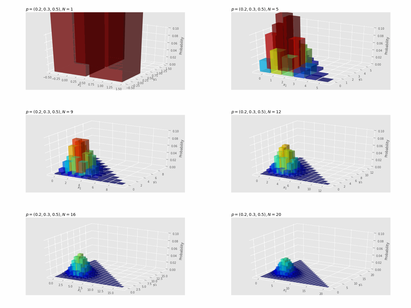
Check the effect of $N
With
import numpy as np
from scipy.stats import multinomial
import matplotlib
import matplotlib.pyplot as plt
from matplotlib import animation, rc
from matplotlib.animation import FuncAnimation

rc('animation', html='html5')
np.random.seed(5)

# Set up formatting for the movie files
Writer = animation.writers['ffmpeg']
writer = Writer(fps=15, metadata=dict(artist='Me'), bitrate=1800)

p_v = np.array([0.2, 0.3, 0.5])
N_max = 20
p_max = 0.1

plt.style.use('ggplot')
cm = plt.get_cmap('jet')
fig = plt.figure(figsize=(10, 5))
ax = fig.add_subplot(projection='3d')

def update(N):
    # initialize previous frame
    plt.cla()

    N += 1

    x_vals = np.arange(N + 1)
    X1, X2 = np.meshgrid(x_vals, x_vals)

    x1_vals = np.delete(X1.flatten(), obj=(X1 + X2).flatten() > N)
    x2_vals = np.delete(X2.flatten(), obj=(X1 + X2).flatten() > N)
    x3_vals = np.where(x1_vals+x2_vals <= N, N - (x1_vals+x2_vals), 0.0)

    x_points = np.stack([x1_vals, x2_vals, x3_vals], axis=1)

    probability = multinomial.pmf(x=x_points, n=N, p=p_v)

    ax.bar3d(x=x1_vals - 0.45,
             y=x2_vals - 0.45,
             z=np.zeros_like(x1_vals),
             dx=0.9,
             dy=0.9,
             dz=probability,
             color=cm(probability / p_max),
             alpha=0.5,
             shade=True
    )
    ax.set_xlabel('$x_1$')
    ax.set_ylabel('$x_2$')
    ax.set_zlabel('Probability')
    ax.set_title('$p=(' + ', '.join([str(phi) for phi in p_v]) + ')' +
                 ', N=' + str(N) + '$', loc='left')
    ax.set_zlim(0.0, p_max)

anime_prob = FuncAnimation(fig, update, frames=N_max, interval=100)

anime_prob.save('multinomial_dist.gif', writer='pillow', fps=1)

As