2022-12-23

Logistic regression

Statistics

Statistical Model

Python

What is logistic regression

Logistic regression is a GLM used to express observed events in terms of a binomial distribution.

The link function of the binomial distribution is often the logit link function, which corresponds to the left side of the following equation.

\log \frac{p_i}{1-p_i}=z_i

where $p_i$ is the probability and $z_i$ is the linear predictor.

Building a logistic regression model

Let us actually construct a logistic regression model. Here we consider seed data for 100 fictitious plants. The data consists of the following columns:

N: Number of seeds
y: Number of germinated seeds
x: Size of the individuals
f: Whether the individuals were treated with fertilizer or not (C: not treated, T: treated)

import pandas as pd

# number of seeds
N = [8,8,8,8,8,8,8,8,8,8,8,8,8,8,8,8,8,8,8,8,8,8,8,8,8,8,8,8,8,8,8,8,8,8,8,8,8,8,8,
     8,8,8,8,8,8,8,8,8,8,8,8,8,8,8,8,8,8,8,8,8,8,8,8,8,8,8,8,8,8,8,8,8,8,8,8,8,8,8,
     8,8,8,8,8,8,8,8,8,8,8,8,8,8,8,8,8,8,8,8,8,8]

# number of seeds germinated
y = [1,6,5,6,1,1,3,6,0,8,0,2,0,5,3,6,3,4,5,8,5,8,1,4,1,8,4,7,5,5,8,1,7,1,3,8,6,7,
     7,4,7,8,8,0,6,5,8,3,8,8,0,5,5,8,3,2,7,8,3,5,8,3,6,7,8,6,5,5,0,8,8,0,6,1,8,8,
     6,6,6,6,8,8,7,8,6,2,0,7,8,8,8,3,7,8,8,7,0,5,8,1]

# body size
x = [9.76,10.48,10.83,10.94,9.37,8.81,9.49,11.02,7.97,11.55,9.46,9.47,8.71,10.42,10.06,
     11,9.95,9.52,10.26,11.33,9.77,10.59,9.35,10,9.53,12.06,9.68,11.32,10.48,10.37,11.33,
     9.42,10.68,7.91,9.39,11.65,10.66,11.23,10.57,10.42,11.73,12.02,11.55,8.58,11.08,10.49,
     11.12,8.99,10.08,10.8,7.83,8.88,9.74,9.98,8.46,7.96,9.78,11.93,9.04,10.14,11.01,8.88,
     9.68,9.8,10.76,9.81,8.37,9.38,7.68,10.23,9.83,7.66,9.33,8.2,9.54,10.55,9.88,9.34,10.38,
     9.63,12.44,10.17,9.29,11.17,9.13,8.79,8.19,10.25,11.3,10.84,10.97,8.6,9.91,11.38,10.39,
     10.45,8.94,8.94,10.14,8.5]

# feed (C: control, T: treatment)
f = ['C','C','C','C','C','C','C','C','C','C','C','C','C','C','C','C','C','C','C','C','C','C',
     'C','C','C','C','C','C','C','C','C','C','C','C','C','C','C','C','C','C','C','C','C','C',
     'C','C','C','C','C','C','T','T','T','T','T','T','T','T','T','T','T','T','T','T','T','T',
     'T','T','T','T','T','T','T','T','T','T','T','T','T','T','T','T','T','T','T','T','T','T',
     'T','T','T','T','T','T','T','T','T','T','T','T']

df = pd.DataFrame(list(zip(N, y, x, f)), columns =['N', 'y', 'x', 'f'])
display(df.head())

	N	y	x	f
0	8	1	9.76	C
1	8	6	10.48	C
2	8	5	10.83	C
3	8	6	10.94	C
4	8	1	9.37	C

Data investigation

Let us check descriptive statistics.

df.describe()

	N	y	x
count	100.0	100.000000	100.000000
mean	8.0	5.080000	9.967200
std	0.0	2.743882	1.088954
min	8.0	0.000000	7.660000
25%	8.0	3.000000	9.337500
50%	8.0	6.000000	9.965000
75%	8.0	8.000000	10.770000
max	8.0	8.000000	12.440000

Displays the number of C and T for f, respectively.

print('num of C:', len(df[df['f'] == 'C']))
print('num of T:', len(df[df['f'] == 'T']))

num of C: 50
num of T: 50

The descriptive statistics of the data confirm the following

Number of seeds N:
- All the numbers are in 8.
Number of germinated seeds y:
- Non-negative integer (0 to 8)
Size of individuals x:
- Positive real numbers (continuous values)
- Variance is small.
Fertilizer treatment f:
- It is categorical data.
- The number of elements in each category is equal.

import matplotlib.pyplot as plt
import seaborn as sns
%matplotlib inline

plt.style.use('ggplot')
plt.figure(figsize=(10,5))
sns.set(rc={'figure.figsize':(10,5)})

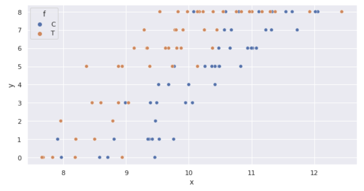
sns.scatterplot(x='x', y='y', hue='f', data=df)

Scatter of f

Displays a box-and-whisker diagram.

sns.boxplot(x='f', y='y', data=df)

Box of f

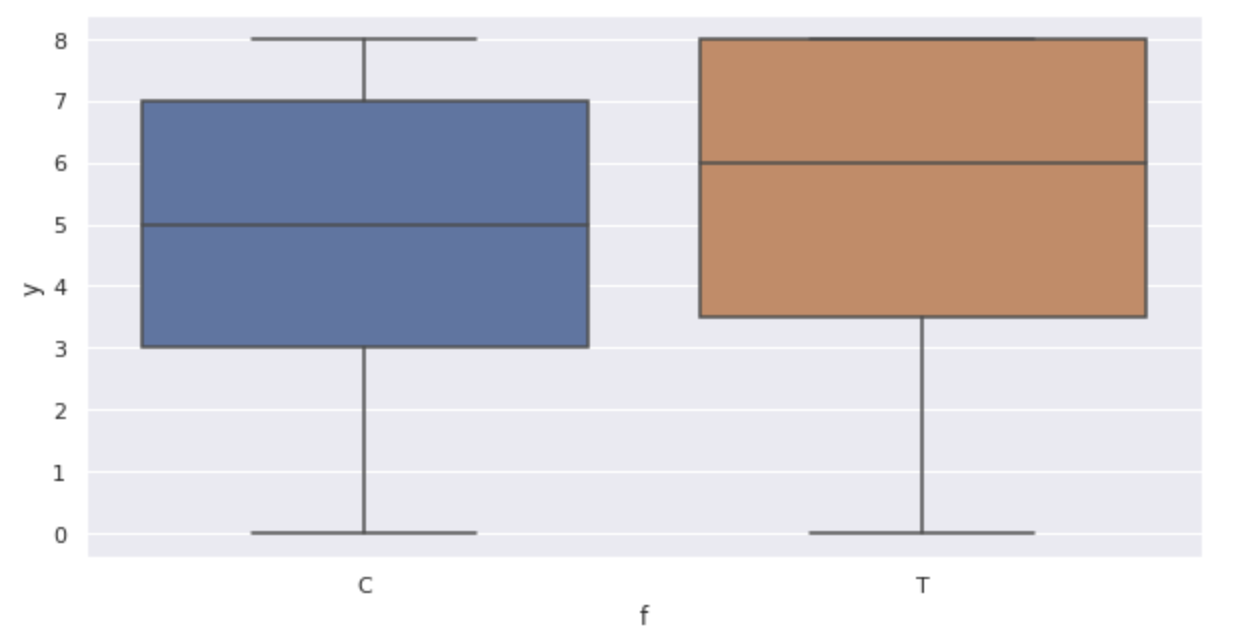
The graph confirms the following:

As $x$ increases in size, the number of germinated seeds y also increases (scatter plot).
The number of germinated seeds y also increases with fertilization (box-and-whisker plot)

Model Building

For $N$ and $y$ of data, we can assume that $N=8$ seeds were extracted, $y$ of the 8 seeds germinated, and $8-y$ seeds did not germinate. The probability distribution often used for such an event is the binomial distribution.

The binomial distribution is represented by the following equation:

P(X = y) = \frac{N!}{y!(N-y)!}p^{y}(1-p)^{N-y}

Let $p$ be the germination probability.

We consider a statistical model in which the germination probability $p_i$ of an individual $i$ is expressed in terms of size $x_i$ and fertilizer treatment $f_i$ .

P(X = y_i) = \frac{N!}{y_i!(N-y_i)!}p^{y_i}(1-p_i)^{N-y_i}

A function often used to express probability is the logistic function. The logistic function is expressed by the following equation:

y = \frac{1}{1 + e^{-x}}

The logistic function is illustrated below.

import matplotlib.pyplot as plt
import pandas as pd
import seaborn as sns
%matplotlib inline

plt.style.use('ggplot')
plt.figure(figsize=(10,5))

x = np.arange(-10, 10, 0.01)
y = [ 1 / ( 1 + math.exp(-x_i))  for x_i in x]
plt.plot(x, y, color='black', label='logsitic function')
plt.xlabel('x')
plt.ylabel('y')
plt.legend()
plt.show()

Logistic function

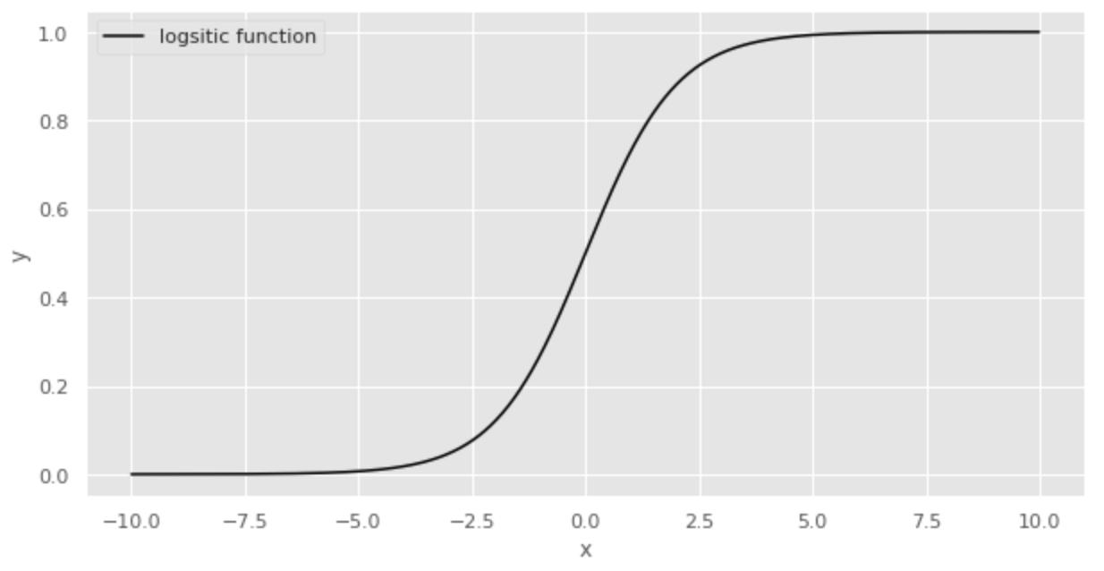
The logistic function ranges from 0 to 1 for y and 0.5 when x is 0. This property makes the logistic function a suitable function for expressing probability.

If we replace the logistic function with the variables in this case, we obtain the following equation.

p_i = \frac{1}{1 + e^{-z_i}}

where $z_i$ is the linear predictor.

The transformation for $z_i$ is as follows.

\log \frac{p_i}{1-p_i}=z_i

The left-hand side of the above equation is called the logit link function. The logit link function is the inverse function of the logistic function.

Expressing the seed germination probability $p_i$ in terms of size $x$ and with/without fertilizer treatment $d$ (dummy variable for fertilizer treatment $f$ ), $z_i$ is as follows:

z_i = \beta_1 + \beta_2 x_i + \beta_3 d_i

That is, the germination probability $p_i$ is as follows:

p_i = \frac{1}{1 + e^{\beta_1 + \beta_2 x_i + \beta_3 d_i}}

Therefore, we are looking for $\beta_1$ , $\beta_2$ , and $\beta_3$ that maximize the following log-likelihood functions:

L(p_i) = \prod^{100}_{i=1} \frac{N!}{y_i!(N-y_i)!}p^{y_i}(1-p_i)^{N-y_i}

Parameter estimation

The $\beta_1$ , $\beta_2$ , and $\beta_3$ can be easily estimated with the following code.

import statsmodels.api as sm
import statsmodels.formula.api as smf

fit_xf = smf.glm(formula='y + I(N - y) ~ x + f', data=df, family=sm.families.Binomial()).fit()
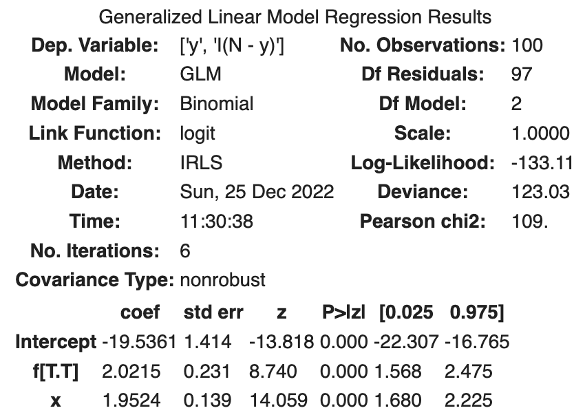
fit_xf.summary()

Poisson regression | f

# aic
fit_xf.aic

The following results were obtained

	coef	std err	z	Log-likelihood	AIC
Intercept	-19.5361	1.414	-13.818
f[T.T]	2.0215	0.231	8.740
x	1.9524	0.139	14.059
				-133.11	272.21

Substitute the estimated parameters into the logistic regression model and illustrate.

import numpy as np
import math

sns.scatterplot(x='x', y='y', hue='f', data=df)
x = np.arange(df.x.min(), df.x.max() + 0.01, 0.01)
y_T = [8 * 1 / ( 1 + math.exp(-(fit_xf.params['Intercept'] + fit_xf.params['x'] * x_i + fit_xf.params['f[T.T]'])))  for x_i in x]
y_C = [8 * 1 / ( 1 + math.exp(-(fit_xf.params['Intercept'] + fit_xf.params['x'] * x_i)))  for x_i in x]
plt.plot(x, y_T, color='black', label='logsitic T')
plt.plot(x, y_C, color='gray', label='logsitic C')
plt.legend()
plt.show()

logistic regression

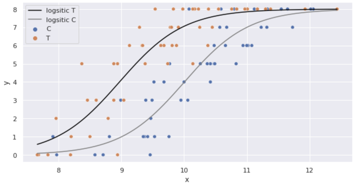
It looks like a good model is being built.

Interpreting logit

Let us transform the logit link function as follows:

\log \frac{p_i}{1 - p_i} = z_i = \beta_1 + \beta_2 x_i + \beta_3 d_i

\frac{p_i}{1 - p_i} = e^{\beta_1 + \beta_2 x_i + \beta_3 d_i} = e^{\beta_1} e^{\beta_2 x_i} e^{\beta_3 d_i}

The left side $\frac{p_i}{1 - p_i}$ is a value called odds, which in this case can be interpreted as (probability of germination)/(probability of not germinating). For example, if $p_i=0.5$ , the odds are 1x.

The odds are proportional to $e^{\textrm{parameter} \times \textrm{factor}}$ . The odds for the presence or absence of fertilizer treatment are as follows