


What is Gamma regression
Gamma regression is a GLM used to express observed events in terms of a gamma distribution. The link function of the gamma distribution is often used with the log link function.
Building gamma regression models
Let us actually construct gamma regression models. In this case, we will use Boston Housing Dataset from scikit-learn.
import pandas as pd
import numpy as np
from sklearn.datasets import load_boston

boston = load_boston()
X = boston.data
y = boston.target

df = pd.DataFrame(X, columns = boston.feature_names).assign(MEDV=np.array(y))
df = df[['RM', 'MEDV']]
display(df.head())
| RM | MEDV | |
|---|---|---|
| 0 | 6.575 | 24.0 |
| 1 | 6.421 | 21.6 |
| 2 | 7.185 | 34.7 |
| 3 | 6.998 | 33.4 |
| 4 | 7.147 | 36.2 |
The meaning of each column is as follows
- MEDV: Median value of owner occupied housing units at $1000
- RM: Average number of rooms per dwelling
Data investigation
Let us check descriptive statistics.
df.describe()
| RM | MEDV | |
|---|---|---|
| count | 506.000000 | 506.000000 |
| mean | 6.284634 | 22.532806 |
| std | 0.702617 | 9.197104 |
| min | 3.561000 | 5.000000 |
| 25% | 5.885500 | 17.025000 |
| 50% | 6.208500 | 21.200000 |
| 75% | 6.623500 | 25.000000 |
| max | 8.780000 | 50.000000 |
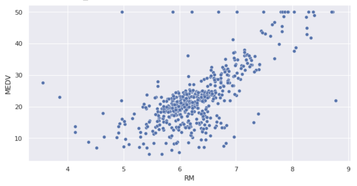
Displays scatter plots.
import matplotlib.pyplot as plt
import seaborn as sns
%matplotlib inline

plt.figure(figsize=(10,5))
sns.set(rc={'figure.figsize':(10,5)})

sns.scatterplot(x='RM', y='MEDV', data=df)
Model building
Assume that the MEDV follows a gamma distribution. In this case, we will construct the following two gamma regression models with the mean MEDV as
| Model | log link function |
|---|---|
| Model 1 | |
| Model 2 |
Parameter estimation (Model 1)
The
import statsmodels.formula.api as smf
import statsmodels.api as sm

fit = smf.glm(formula='MEDV ~ RM', data=df, family=sm.families.Gamma(link=sm.families.links.log)).fit()
fit.summary()
The following results were obtained.
| GLM Results | |||
|---|---|---|---|
| Dep. Variable | MEDV | No. Observations | 506 |
| Model | GLM | Df Residuals | 504 |
| Model Family | Gamma | Df Model | 1 |
| Link Function | log | Scale: | 0.096893 |
| Method | IRLS | Log-Likelihood | -1658.9 |
| Date | Wed, 28 Dec 2022 | Deviance: | 47.467 |
| Time | 02:50:46 | Pearson chi2 | 48.8 |
| No. Iterations | 15 | Covariance Type | nonrobust |
| coef | std err | z | P>|z| | [0.025 | 0.975] | |
|---|---|---|---|---|---|---|
| Intercept | 0.9379 | 0.125 | 7.524 | 0.000 | 0.694 | 1.182 |
| RM | 0.3411 | 0.020 | 17.300 | 0.000 | 0.302 | 0.380 |
Let us derive AIC.
fit.aic

3321.8747164073784
Substitute the estimated parameters into the gamma regression model and illustrate.
import numpy as np
import math

sns.scatterplot(x='RM', y='MEDV', data=df)
x = np.arange(df.RM.min(), df.RM.max() + 0.01, 0.01)
y = np.exp(fit.params['Intercept'] + fit.params['RM'] * x)
y_lower = np.exp((fit.conf_int().loc['Intercept'][0]) + fit.conf_int().loc['RM'][0] * x)
y_upper = np.exp((fit.conf_int().loc['Intercept'][1]) + fit.conf_int().loc['RM'][1] * x)
plt.plot(x, y, color='black', label='gamma regression')
plt.fill_between(x, y_lower, y_upper, color='grey', alpha=0.2, label='95% confidence interval')
plt.legend()
plt.show()
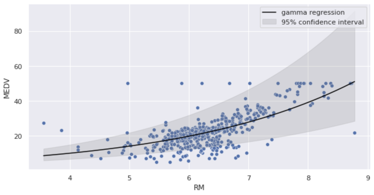
Since it is a log link function, we can see that the curve is predicted to be a right shoulder curve.
Parameter estimation (Model 2)
Parameters glm function formula is written as formula='MEDV ~ np.log(RM)'.
import statsmodels.formula.api as smf
import statsmodels.api as sm

fit = smf.glm(formula='MEDV ~ np.log(RM)', data=df, family=sm.families.Gamma(link=sm.families.links.log)).fit()
fit.summary()
| GLM Results | |||
|---|---|---|---|
| Dep. Variable | MEDV | No. Observations | 506 |
| Model | GLM | Df Residuals | 504 |
| Model Family | Gamma | Df Model | 1 |
| Link Function | log | Scale: | 0.10838 |
| Method | IRLS | Log-Likelihood | -1675.8 |
| Date | Wed, 28 Dec 2022 | Deviance: | 50.505 |
| Time | 02:50:46 | Pearson chi2 | 54.6 |
| No. Iterations | 22 | Covariance Type | nonrobust |
| coef | std err | z | P>|z| | [0.025 | 0.975] | |
|---|---|---|---|---|---|---|
| Intercept | -0.5489 | 0.239 | -2.293 | 0.022 | -1.018 | -0.080 |
| np.log(RM) | 1.9834 | 0.130 | 15.208 | 0.000 | 1.728 | 2.239 |
Let us derive the AIC.
fit.aic

3355.6367279321394
The AIC is larger than in Model 1.
Let us substitute the estimated parameters into the gamma regression model and illustrate.
import numpy as np
import math

sns.scatterplot(x='RM', y='MEDV', data=df)
x = np.arange(df.RM.min(), df.RM.max() + 0.01, 0.01)
y = np.exp(fit.params['Intercept'] + fit.params['np.log(RM)'] * np.log(x))
y_lower = np.exp((fit.conf_int().loc['Intercept'][0]) + fit.conf_int().loc['np.log(RM)'][0] * np.log(x))
y_upper = np.exp((fit.conf_int().loc['Intercept'][1]) + fit.conf_int().loc['np.log(RM)'][1] * np.log(x))
plt.plot(x, y, color='black', label='gamma regression')
plt.fill_between(x, y_lower, y_upper, color='grey', alpha=0.2, label='95% confidence interval')
plt.legend()
plt.show()
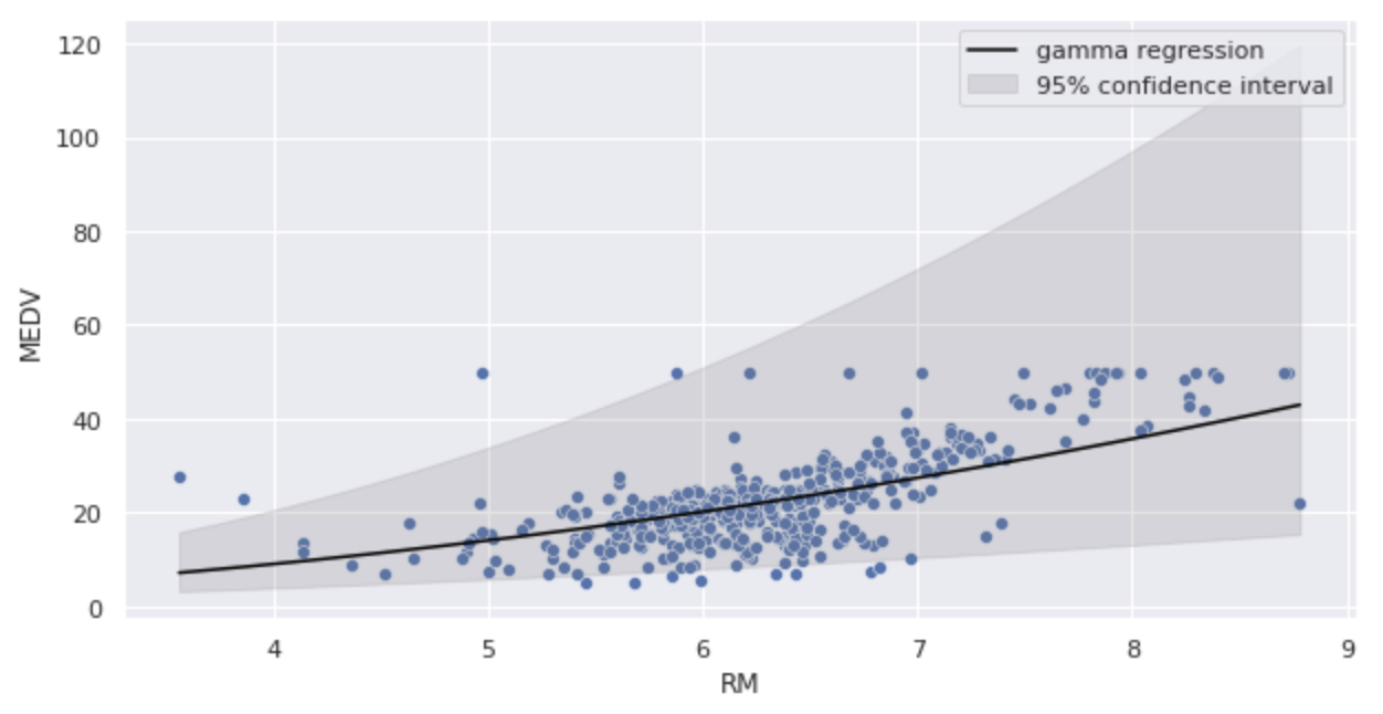
The slope of the curve is more gradual than in Model 1.


Ryusei Kakujo


Weave the future of cities through data
Transportation modeling/ Urban planning/ Machine learning/ Computer science/ GIS