2022-12-23

Generalized linear mixed model

What is Generalized Linear Mixed Model (GLMM)

Generalized Linear Mixed Model (GLMM) is a statistical model that is a further development of GLM. It can represent unobservable individual and regional differences.

Unobservable individual and regional differences include, for example, the following:

Individual differences in pain perception
Different people respond differently to the same pain.
Individual differences in scoring
Some scorers are more lenient than others.
Regional differences
There are regional variations in the nature of the pain.

A model that does not account for these individual and regional differences will lead to overdispersion. Overdispersion means that the assumed probability distribution has a larger variance than assumed. The following figure shows overdispersion using the Poisson distribution as an example.

Overdispersion

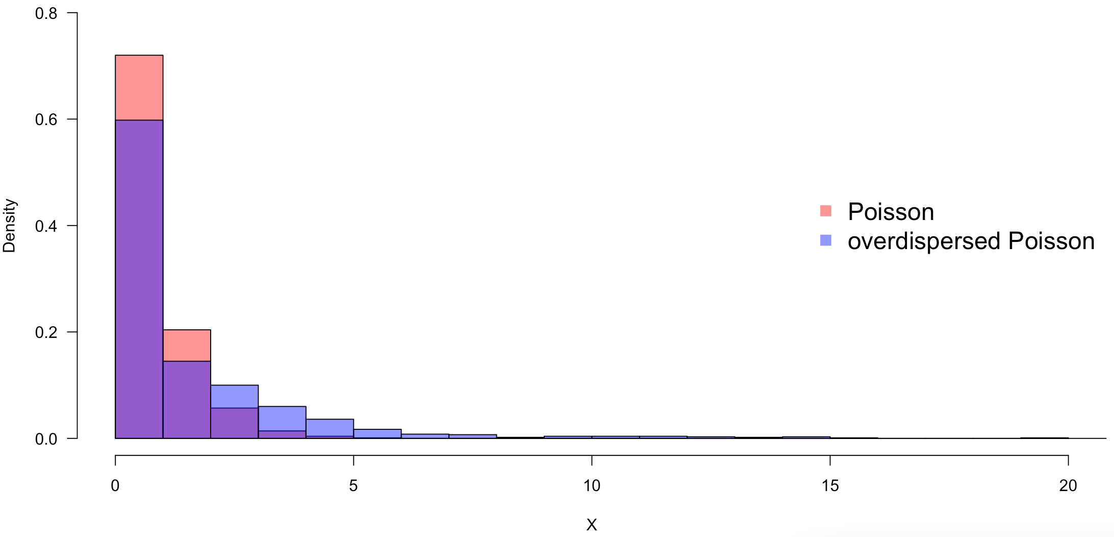
Individual and regional differences can result in a Poisson distribution that is larger than the original Poisson distribution, as in the case of overdispersed Poisson, and without taking individual and location differences into account, the observed data cannot be modeled well.

GLMM treats unexplained variation such as individual and location differences as random effects and models them as such, with determining that it is impossible to observe all of the explanatory variables.

Random Effects

GLMM adds random effects to linear predictors. For example, for individual $i$ , add individual differences as random effects $\eta_i$ as follows:

g(y_i) = \beta_1 + \beta_2 x_i + \cdots + \eta_i

We assume that the random effect $\eta_i$ follows a normal distribution with mean 0 and variance $s$ . There is no reason to assume that the distribution of $\eta_i$ follows a normal distribution, but it is assumed to be a normal distribution because it is convenient for statistical modeling.

Maximum likelihood estimation of the parameters will be done for $\beta$ and $s$ .

Cases where GLMM is required

The criterion for determining whether a GLMM is necessary is whether you are sampling the same individuals or locations over and over again. For example, GLMM is often applied to panel data, which are data observed repeatedly over time for individuals.

Build GLMM

Let us construct a GLMM using the dataset grouseticks. grouseticks is an observation of the number of ticks on the heads of red grouse chicks and consists of the following columns:

INDEX: (factor) chick number (observation level)
TICKS: number of ticks sampled
BROOD: (factor) brood number
HEIGHT: height above sea level (meters)
YEAR: year (-1900)
LOCATION: (factor) geographic location code
cHEIGHT: centered height, derived from HEIGHT

Let us check the data.

> require(lme4)
> library(lme4)
> data(grouseticks)
> summary(grouseticks)

    INDEX         TICKS           BROOD         HEIGHT      YEAR        LOCATION      cHEIGHT
1      :  1   Min.   : 0.00   606    : 10   Min.   :403.0   95:117   14     : 24   Min.   :-59.241
2      :  1   1st Qu.: 0.00   602    :  9   1st Qu.:430.0   96:155   4      : 20   1st Qu.:-32.241
3      :  1   Median : 2.00   537    :  7   Median :457.0   97:131   19     : 20   Median : -5.241
4      :  1   Mean   : 6.37   601    :  7   Mean   :462.2            28     : 19   Mean   :  0.000
5      :  1   3rd Qu.: 6.00   643    :  7   3rd Qu.:494.0            50     : 17   3rd Qu.: 31.759
6      :  1   Max.   :85.00   711    :  7   Max.   :533.0            36     : 16   Max.   : 70.759
(Other):397                   (Other):356                            (Other):287

> head(grouseticks)

  INDEX TICKS BROOD HEIGHT YEAR LOCATION   cHEIGHT
1     1     0   501    465   95       32  2.759305
2     2     0   501    465   95       32  2.759305
3     3     0   502    472   95       36  9.759305
4     4     0   503    475   95       37 12.759305
5     5     0   503    475   95       37 12.759305
6     6     3   503    475   95       37 12.759305

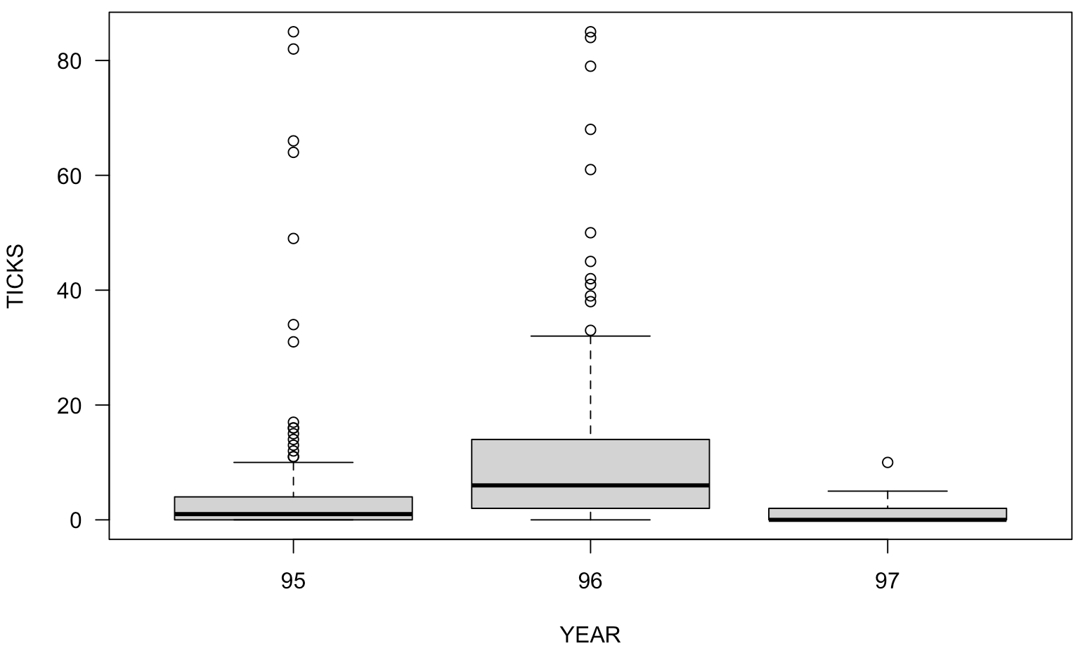
> plot(TICKS ~ HEIGHT, las=1)

TICKS and HEIGHT

Poisson regression without random effects

This time we will construct a Poisson regression model. Using the average number of ticks $\lambda_i$ we express the log-link function as follows

\log \lambda_i = \beta_1 + \beta_2 d_i

where $d_i$ is a dummy variable for Year.

The following code can be used to estimate the parameters.

> fit_glm <- glm(TICKS ~ YEAR, family=poisson(), data=grouseticks)
> summary)(fit_glm)

Call:
glm(formula = TICKS ~ YEAR, family = poisson(), data = grouseticks)

Deviance Residuals:
    Min       1Q   Median       3Q      Max
-4.7110  -2.8888  -1.5183   0.7139  17.1467

Coefficients:
            Estimate Std. Error z value Pr(>|z|)
(Intercept)  1.78318    0.03790   47.05   <2e-16 ***
YEAR96       0.62348    0.04492   13.88   <2e-16 ***
YEAR97      -1.64109    0.08977  -18.28   <2e-16 ***
---
Signif. codes:  0 ‘***’ 0.001 ‘**’ 0.01 ‘*’ 0.05 ‘.’ 0.1 ‘ ’ 1

(Dispersion parameter for poisson family taken to be 1)

    Null deviance: 5847.5  on 402  degrees of freedom
Residual deviance: 4549.4  on 400  degrees of freedom
AIC: 5486.4

Number of Fisher Scoring iterations: 6

AIC is 5486.4.

Poisson regression with random effects

let us construct a Poisson regression model with random effects.

Random intercept model

Add the random effect $\eta_j$ of location $j$ by LOCATION and express the average number of ticks $\lambda_i$ as follows.

\log \lambda_i = \beta_1 + \beta_2 d_i + \eta_j, \quad \eta_j \sim N(0, s^2)

This model is also called the random intercept model because random effects are included in the intercept.

You can estimate $\beta$ and $S$ with the following code. If you want random effects in the intercept, write TICKS ~ YEAR + (1 | LOCATION).

> fit_glmm <- glmer(TICKS ~ YEAR + (1 | LOCATION), family="poisson", data=grouseticks)
> summary(fit_glmm)

Generalized linear mixed model fit by maximum likelihood (Laplace Approximation) ['glmerMod']
 Family: poisson  ( log )
Formula: TICKS ~ YEAR + (1 | LOCATION)
   Data: grouseticks

     AIC      BIC   logLik deviance df.resid
  2306.3   2322.3  -1149.1   2298.3      399

Scaled residuals:
    Min      1Q  Median      3Q     Max
-6.6399 -0.8844 -0.4708  0.8543  5.5757

Random effects:
 Groups   Name        Variance Std.Dev.
 LOCATION (Intercept) 1.644    1.282
Number of obs: 403, groups:  LOCATION, 63

Fixed effects:
            Estimate Std. Error z value Pr(>|z|)
(Intercept)  0.64992    0.18319   3.548 0.000388 ***
YEAR96       0.94371    0.08492  11.113  < 2e-16 ***
YEAR97      -1.43642    0.12298 -11.681  < 2e-16 ***
---
Signif. codes:  0 ‘***’ 0.001 ‘**’ 0.01 ‘*’ 0.05 ‘.’ 0.1 ‘ ’ 1

Correlation of Fixed Effects:
       (Intr) YEAR96
YEAR96 -0.295
YEAR97 -0.241  0.520

The AIC is now 2306.3, a significant improvement over the model without random effects.

The variance of random effects for LOCATION is 1.644. You can check the random effects of all LOCATION with the randf() function.

> ranef(fit_glmm)

$LOCATION
   (Intercept)
1   1.24539318
2   0.92293852
3  -0.93190888
.
.
.
61 -1.35144088
62 -0.95446024
63 -1.15277383

with conditional variances for “LOCATION”

The values from 1 to 63 are the LOCATION values: intercept for 1 is 1.24539318 and intercept for 3 is -0.93190888. The interpretation is that LOCATION 1 has relatively more ticks than LOCATION 3.

In addition, a random effect $\tau_i$ due to INDEX can be added.

\log \lambda_i = \beta_1 + \beta_2 d_i + \eta_j + \tau_i, \quad \eta_j \sim N(0, s^2), \tau_i \sim N(0, \sigma^2)

> fit_glmm <- glmer(TICKS ~ YEAR + (1 | LOCATION) + (1 | INDEX), family="poisson", data=grouseticks)
> summary(fit_glmm)

Generalized linear mixed model fit by maximum likelihood (Laplace Approximation) ['glmerMod']
 Family: poisson  ( log )
Formula: TICKS ~ YEAR + (1 | LOCATION) + (1 | INDEX)
   Data: grouseticks

     AIC      BIC   logLik deviance df.resid
  1863.9   1883.9   -927.0   1853.9      398

Scaled residuals:
    Min      1Q  Median      3Q     Max
-1.5003 -0.5933 -0.1154  0.2723  2.3743

Random effects:
 Groups   Name        Variance Std.Dev.
 INDEX    (Intercept) 0.5081   0.7128
 LOCATION (Intercept) 1.4679   1.2116
Number of obs: 403, groups:  INDEX, 403; LOCATION, 63

Fixed effects:
            Estimate Std. Error z value Pr(>|z|)
(Intercept)   0.2774     0.2107   1.316    0.188
YEAR96        1.2578     0.1821   6.906 4.97e-12 ***
YEAR97       -1.0856     0.2010  -5.400 6.67e-08 ***
---
Signif. codes:  0 ‘***’ 0.001 ‘**’ 0.01 ‘*’ 0.05 ‘.’ 0.1 ‘ ’ 1

Correlation of Fixed Effects:
       (Intr) YEAR96
YEAR96 -0.536
YEAR97 -0.439  0.552

The AIC is now 1863.9, which is a further improvement.

The variance of random effects for LOCATION is 1.4679 and for INDEX is 0.5081. We can see that the random effect of INDEX is smaller than that of LOCATION.

Random coefficient model

Let us add the random effect $\eta_j$ by LOCATION not only to the intercept but also to the coefficient.

\log \lambda_i = (\beta_1 + \eta_{1j}) + (\beta_2 + \eta_{2j}), \quad \eta_{1j} \sim N(0, s^2), \quad \eta_{2j} \sim N(0, \sigma^2)

This model is also called the random coefficient model because random effects are included in the coefficients.

The following code can estimate $\beta$ , $s$ , and $\sigma$ . To include random effects in the intercept and coefficients, you can write TICKS ~ YEAR + (YEAR | LOCATION).

> fit_glmm <- glmer(TICKS ~ YEAR + (YEAR | LOCATION), family="poisson", data=grouseticks)
> summary(fit_glmm)

Generalized linear mixed model fit by maximum likelihood (Laplace Approximation) ['glmerMod']
 Family: poisson  ( log )
Formula: TICKS ~ YEAR + (YEAR | LOCATION)
   Data: grouseticks

     AIC      BIC   logLik deviance df.resid
  2266.7   2302.7  -1124.3   2248.7      394

Scaled residuals:
    Min      1Q  Median      3Q     Max
-6.6442 -0.8112 -0.4797  0.8437  5.5779

Random effects:
 Groups   Name        Variance Std.Dev. Corr
 LOCATION (Intercept) 2.3583   1.5357
          YEAR96      0.6002   0.7747   -0.70
          YEAR97      0.6735   0.8207   -0.80  0.46
Number of obs: 403, groups:  LOCATION, 63

Fixed effects:
            Estimate Std. Error z value Pr(>|z|)
(Intercept)   0.3273     0.2674   1.224  0.22083
YEAR96        1.3094     0.2542   5.152 2.58e-07 ***
YEAR97       -0.7578     0.2909  -2.605  0.00918 **
---
Signif. codes:  0 ‘***’ 0.001 ‘**’ 0.01 ‘*’ 0.05 ‘.’ 0.1 ‘ ’ 1

Correlation of Fixed Effects:
       (Intr) YEAR96
YEAR96 -0.746
YEAR97 -0.668  0.553

However, this estimation is for a model that assumes the correlation between $\eta_{1j}$ and $\eta_{2j}$ . If you want to fit a model assuming that both parameters are independent of each other, write TICKS ~ YEAR + (1 | LOCATION) + (0 + YEAR | LOCATION).

> fit_glmm <- glmer(TICKS ~ YEAR + (1 | LOCATION) + (0 + YEAR | LOCATION), family="poisson", data=grouseticks)
> summary(fit_glmm)

Generalized linear mixed model fit by maximum likelihood (Laplace Approximation) ['glmerMod']
 Family: poisson  ( log )
Formula: TICKS ~ YEAR + (1 | LOCATION) + (0 + YEAR | LOCATION)
   Data: grouseticks

     AIC      BIC   logLik deviance df.resid
  2268.7   2308.7  -1124.3   2248.7      393

Scaled residuals:
    Min      1Q  Median      3Q     Max
-6.6442 -0.8112 -0.4797  0.8437  5.5779

Random effects:
 Groups     Name        Variance Std.Dev. Corr
 LOCATION   (Intercept) 0.4151   0.6443
 LOCATION.1 YEAR95      1.9431   1.3939
            YEAR96      0.8755   0.9357   0.85
            YEAR97      0.6006   0.7750   0.87 0.54
Number of obs: 403, groups:  LOCATION, 63

Fixed effects:
            Estimate Std. Error z value Pr(>|z|)
(Intercept)   0.3274     0.2674   1.224  0.22081
YEAR96        1.3094     0.2542   5.152 2.58e-07 ***
YEAR97       -0.7578     0.2909  -2.605  0.00918 **
---
Signif. codes:  0 ‘***’ 0.001 ‘**’ 0.01 ‘*’ 0.05 ‘.’ 0.1 ‘ ’ 1

Correlation of Fixed Effects:
       (Intr) YEAR96
YEAR96 -0.746
YEAR97 -0.668  0.553

It is also possible to add random effects only to coefficients by writing TICKS ~ YEAR + (0 + YEAR | LOCATION).

> fit_glmm <- glmer(TICKS ~ YEAR + (0 + YEAR | LOCATION), family="poisson", data=grouseticks)

Warning message:
In checkConv(attr(opt, "derivs"), opt$par, ctrl = control$checkConv,  :
  Model failed to converge with max|grad| = 0.0139508 (tol = 0.002, component 1)

> summary(fit_glmm)

Generalized linear mixed model fit by maximum likelihood (Laplace Approximation) ['glmerMod']
 Family: poisson  ( log )
Formula: TICKS ~ YEAR + (0 + YEAR | LOCATION)
   Data: grouseticks

     AIC      BIC   logLik deviance df.resid
  2266.7   2302.7  -1124.3   2248.7      394

Scaled residuals:
    Min      1Q  Median      3Q     Max
-6.6442 -0.8114 -0.4793  0.8432  5.5778

Random effects:
 Groups   Name   Variance Std.Dev. Corr
 LOCATION YEAR95 2.363    1.537
          YEAR96 1.291    1.136    0.87
          YEAR97 1.016    1.008    0.87 0.70
Number of obs: 403, groups:  LOCATION, 63

Fixed effects:
            Estimate Std. Error z value Pr(>|z|)
(Intercept)   0.3276     0.2676   1.224  0.22093
YEAR96        1.3099     0.2543   5.151 2.59e-07 ***
YEAR97       -0.7566     0.2908  -2.601  0.00929 **
---
Signif. codes:  0 ‘***’ 0.001 ‘**’ 0.01 ‘*’ 0.05 ‘.’ 0.1 ‘ ’ 1

Correlation of Fixed Effects:
       (Intr) YEAR96
YEAR96 -0.746
YEAR97 -0.669  0.554
optimizer (Nelder_Mead) convergence code: 0 (OK)
Model failed to converge with max|grad| = 0.0139508 (tol = 0.002, component 1)

R code

The R code to illustrate the Poisson distribution overdispersion is shown below.

> set.seed(1)
> hist(Y1 <- rpois(1000, 1), breaks=seq(0, 20), col="#FF00007F", freq=F, ylim=c(0, 0.8), las=1,
     main="", xlab="X")
> hist(Y2 <- rpois(1000, 1 * exp(rnorm(1000, mean=0, sd=1))), col="#0000FF7F", add=T, freq=F, breaks=seq(0, 100))
> legend("right", legend=c("Poisson", "overdispersed Poisson"), pch=15, col=c("#FF00007F", "#0000FF7F"),
       bty="n", cex=1.5)