Introduction

Weight initialization is a crucial aspect of training deep learning models, as it can significantly influence the model's performance, training time, and stability. The initial weights of a neural network can impact how quickly the model converges during training and whether it converges to an optimal or suboptimal solution. Choosing the right weight initialization strategy is essential for achieving the best possible results in your deep learning projects.

Weight initialization sets the stage for the learning process by determining the initial values of the weights in a neural network. Proper weight initialization can lead to faster convergence and improved generalization, while poor initialization can result in slow convergence or even the failure to learn. By understanding the impact of different weight initialization techniques, practitioners can make more informed decisions and develop better models.

Techniques for Weight Initialization

In this chapter, I will explore various weight initialization techniques that are widely used in the deep learning community. Each technique has its unique advantages and is suited for different types of neural network architectures and activation functions. Understanding these methods will help you make informed decisions when designing and training your deep learning models.

Zero Initialization

Zero initialization is the simplest method, where all the weights in the network are initialized to zero. Although easy to implement, this approach has a significant downside: all neurons in the network learn the same features during training. As a result, the model becomes unable to capture the complexity of the data, leading to poor performance. This phenomenon is known as the "symmetry problem," and it is generally not recommended to use zero initialization for deep learning models.

Random Initialization

To overcome the symmetry problem, random initialization assigns small random values to the weights. This method ensures that each neuron learns different features, thus enabling the model to capture the complexity of the data. However, random initialization is not without its issues. When the initial weights are too large or too small, it can result in vanishing or exploding gradients, which can negatively impact the learning process.

Xavier (Glorot) Initialization

Proposed by Glorot and Bengio in 2010, Xavier initialization addresses the problems associated with random initialization by scaling the initial weights based on the number of input and output units in a layer. Specifically, the weights are sampled from a Gaussian distribution with mean 0 and variance \frac{2}{n_{in} + n_{out}}, where n_{in} and n_{out} are the number of input and output units, respectively. Xavier initialization works particularly well for networks with sigmoid or hyperbolic tangent (tanh) activation functions.

He (Kaiming) Initialization

He initialization, also known as Kaiming initialization, was introduced by He et al. in 2015. Like Xavier initialization, He initialization also scales the initial weights, but it is specifically designed for networks with Rectified Linear Unit (ReLU) and its variants as activation functions. The weights are sampled from a Gaussian distribution with mean 0 and variance \frac{2}{n_{in}}, where n_{in} is the number of input units in a layer.

LeCun Initialization

LeCun initialization, proposed by Yann LeCun, is another popular weight initialization method. Similar to Xavier and He initialization, LeCun initialization also scales the initial weights based on the layer's input size. The weights are sampled from a Gaussian distribution with mean 0 and variance \frac{1}{n_{in}}. LeCun initialization is well-suited for networks with sigmoid or hyperbolic tangent activation functions.

Orthogonal Initialization

Orthogonal initialization, introduced by Saxe et al. in 2013, initializes the weight matrix with random orthogonal matrices. This method helps preserve the gradient magnitude during backpropagation, which can lead to faster convergence and improved performance. Orthogonal initialization is particularly useful for deep or recurrent neural networks, where vanishing or exploding gradients can be an issue.

Choosing the Right Initialization Method

Selecting the right weight initialization method is essential for training effective deep learning models. In this chapter, I will discuss the factors to consider when choosing an initialization technique, as well as guidelines for selecting the most suitable method for your specific use case.

Network Architecture

The architecture of your neural network plays a critical role in determining the most suitable weight initialization method. For instance, deep networks with many layers are more prone to vanishing or exploding gradients, making techniques like Xavier, He, or Orthogonal initialization more suitable. In contrast, shallow networks might not be as sensitive to the choice of initialization method.

Activation Functions

The type of activation function used in your neural network also influences the choice of weight initialization. For example:

• Sigmoid or Hyperbolic Tangent (tanh) activation functions work well with Xavier or LeCun initialization.
• ReLU and its variants, such as Leaky ReLU and Parametric ReLU, are better suited for He (Kaiming) initialization.
• Deep or recurrent neural networks with a risk of vanishing or exploding gradients can benefit from Orthogonal initialization.

Problem Complexity

The complexity of the problem being solved also plays a role in selecting the appropriate weight initialization method. More complex problems, such as high-dimensional data or tasks with multiple modalities, may require more sophisticated initialization techniques to ensure effective learning.

Selecting the Right Initialization Method

Based on the factors mentioned above, the following guidelines can help you choose the most appropriate weight initialization technique for your deep learning model:

• Avoid zero initialization, as it leads to the symmetry problem and poor model performance.
• For networks with sigmoid or tanh activation functions, consider using Xavier or LeCun initialization.
• For networks with ReLU or its variants, He (Kaiming) initialization is generally the preferred choice.
• For deep or recurrent networks prone to vanishing or exploding gradients, Orthogonal initialization can be a suitable option.

Keep in mind that these are general guidelines, and the best weight initialization method for your specific problem may vary. It is essential to experiment with different techniques and monitor their impact on model performance during the training process.

Comparing Weight Initialization Techniques

In this chapter, I will compare the weight initialization techniques by implementing them in Python and analyzing their impact on the activation distribution of 4-hidden-layer neural network. We will use a public dataset and visualize the activation distribution in the form of histograms to better understand the differences between the initialization methods.

Dataset and Model Setup:

For this comparison, we will use the popular MNIST dataset, which consists of 60,000 training and 10,000 test images of handwritten digits (0-9). We will use a simple feedforward neural network with 5 layers and ReLU activation functions.

The model is a 5-layer neural network with the following structure:

1. Input layer with 784 nodes (corresponding to the flattened MNIST image size of 28x28 pixels)
2. First hidden layer with 512 nodes
3. Second hidden layer with 256 nodes
4. Third hidden layer with 128 nodes
5. Fourth hidden layer with 64 nodes

Implementing Weight Initialization Techniques in Python

Let's start by importing the necessary libraries and defining the initialization functions:

import numpy as np
import matplotlib.pyplot as plt
from keras.datasets import mnist
from keras.models import Sequential
from keras.layers import Dense
from keras.optimizers import Adam
from keras.initializers import Zeros, RandomNormal, GlorotNormal, HeNormal, LecunNormal

# Define weight initialization functions
def init_zeros(shape, dtype=None):
    return Zeros()(shape, dtype=dtype)

def init_random_normal(shape, dtype=None):
    return RandomNormal(stddev=0.01)(shape, dtype=dtype)

def init_xavier(shape, dtype=None):
    return GlorotNormal()(shape, dtype=dtype)

def init_he(shape, dtype=None):
    return HeNormal()(shape, dtype=dtype)

def init_lecun(shape, dtype=None):
    return LecunNormal()(shape, dtype=dtype)

Building the Model and Visualizing Activation Distributions

Now, let's create a function to build the model using the specified weight initialization method, train it on the MNIST dataset, and draw histograms of the activation distribution at each layer.

def build_and_train_model(init_func, dataset, layer_dims=[784, 512, 256, 128, 64], activation='relu', epochs=5):
    (X_train, y_train), (X_test, y_test) = dataset
    model = Sequential()
    input_dim = layer_dims[0]

    for layer_dim in layer_dims[1:]:
        model.add(Dense(layer_dim, input_dim=input_dim, activation=activation, kernel_initializer=init_func))
        input_dim = layer_dim

    model.compile(optimizer=Adam(), loss='sparse_categorical_crossentropy', metrics=['accuracy'])
    history = model.fit(X_train, y_train, epochs=epochs, validation_data=(X_test, y_test), verbose=0)

    activations = []
    for layer in model.layers:
        intermediate_model = Sequential(model.layers[:model.layers.index(layer) + 1])
        activations.append(intermediate_model.predict(X_test))

    return history, activations

Analyzing Activation Distributions

Now let's analyze the activation distributions for each initialization method by plotting histograms at each layer.

initializers = {
    'Zero': init_zeros,
    'Random Normal': init_random_normal,
    'Xavier': init_xavier,
    'He': init_he,
    'LeCun': init_lecun
}

dataset = mnist.load_data()
fig, axes = plt.subplots(len(initializers), 4, figsize=(25, 25))
plt.style.use('ggplot')

for idx, (name, init_func) in enumerate(initializers.items()):
    _, activations = build_and_train_model(init_func, dataset)
    for layer_idx, activation in enumerate(activations):
        axes[idx, layer_idx].hist(activation.flatten(), bins=50, density=True, color='blue', alpha=0.5)
        axes[idx, layer_idx].set_xlim(-1, 1)
        axes[idx, layer_idx].set_ylim(0, 4)
        axes[idx, layer_idx].set_title(f'{name} Initialization - Layer {layer_idx + 1}', fontsize=16)
        axes[idx, layer_idx].set_xlabel('Activation Value', fontsize=12)
        axes[idx, layer_idx].set_ylabel('Density', fontsize=12)

plt.subplots_adjust(hspace=0.4, wspace=0.4)
plt.show()

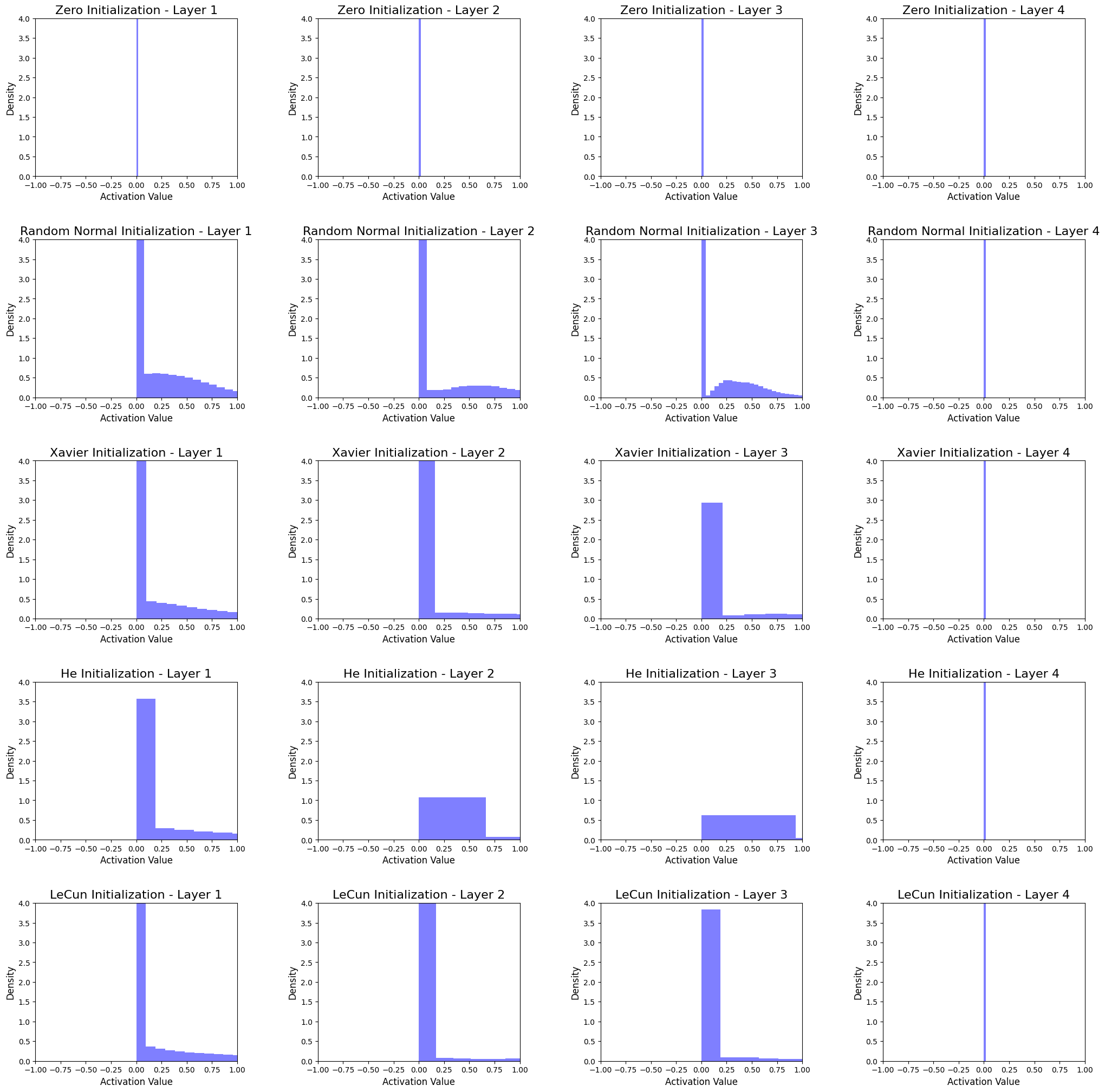
Interpreting the Histograms

The histograms show the activation distributions of the 4-hidden-layer neural network for each initialization method. By analyzing the histograms, we can draw the following conclusions:

• Zero Initialization
  The activations for all layers are concentrated at zero. This shows that the model is unable to capture the complexity of the data and results in poor learning.

• Random Normal Initialization
  The activations at each layer have a normal distribution. However, the majority of the activations are close to zero, which might lead to dead neurons, negatively affecting the learning process.

• Xavier Initialization
  The activations have a normal distribution with a higher standard deviation than Random Normal Initialization, resulting in better learning. This method works well with networks using sigmoid or tanh activation functions, but might not be the best choice for ReLU activation functions.

• He Initialization
  The activations are more evenly spread compared to other methods, which helps avoid dead neurons and leads to better learning. This method is specifically designed for networks with ReLU activation functions and is generally the preferred choice.

• LeCun Initialization
  The activations are similar to those of Xavier Initialization, but with a slightly lower standard deviation. This method is well-suited for networks with sigmoid or tanh activation functions.

In all methods, activations for last hidden layers are concentrated at zero. One of factors may be the node size (64 nodes) at last hidden layer.

From the analysis, we can see that the choice of weight initialization method has a significant impact on the distribution of activations in the network. In general, He Initialization performs the best for networks with ReLU activation functions, while Xavier or LeCun Initialization may be more suitable for networks with sigmoid or tanh activation functions. It is essential to select an appropriate weight initialization technique based on the specific characteristics of your neural network architecture and activation functions.