What is Batch Normalization

Batch normalization is a transformative technique in deep learning that accelerates training, improves model convergence, and simplifies the process of selecting optimal learning rates and weight initialization. Proposed by Ioffe and Szegedy in 2015, batch normalization addresses the problem of internal covariate shift, which occurs when the distribution of the inputs to a given layer in a neural network changes during training due to parameter updates.

The primary goal of batch normalization is to stabilize the input distribution for each layer in a neural network, allowing for faster and more stable training. This is achieved by normalizing the activations of each layer using the mean and variance of each feature within a mini-batch. After normalization, the data is scaled and shifted using learnable parameters that are updated during training. This ensures that the model can still represent a wide range of input distributions.

Importance of Batch Normalization

The introduction of batch normalization has significantly impacted the field of deep learning, as it has become a standard component in the design of various deep learning architectures. The technique offers several benefits that contribute to its widespread adoption:

• Faster training
  By stabilizing input distributions, batch normalization allows for the use of higher learning rates, which speeds up the training process.

• Improved model convergence
  Normalizing layer activations helps prevent the vanishing and exploding gradient problems, which can impede model convergence.

• Reduced sensitivity to initialization
  Batch normalization mitigates the effects of poor weight initialization, making it easier to train deep networks.

• Better generalization
  The regularization effect of batch normalization can help prevent overfitting and improve model generalization on unseen data.

• Simplified hyperparameter tuning
  As batch normalization stabilizes training, it reduces the need for extensive hyperparameter tuning, saving time and computational resources.

Batch normalization has been instrumental in improving the performance of many state-of-the-art models, particularly in computer vision tasks such as image classification, object detection, and semantic segmentation. Moreover, the technique has inspired the development of other normalization methods, such as layer normalization, instance normalization, and group normalization, which have found applications in various domains, including natural language processing and reinforcement learning.

Background and Theory

Covariate Shift

Covariate shift refers to the change in the distribution of input features during the training process. This phenomenon is particularly problematic in deep learning, as it can lead to the internal covariate shift, where the distribution of inputs to each layer changes as the parameters of the preceding layers are updated. The internal covariate shift can slow down training, as it requires lower learning rates and careful initialization to maintain stability.

Batch normalization addresses the issue of internal covariate shift by ensuring that the input distribution to each layer remains consistent throughout training. This is achieved by normalizing the activations of each layer, effectively stabilizing the learning process and enabling the use of higher learning rates.

The Batch Normalization Algorithm

Batch normalization is applied to the activations of each layer before the activation function is applied. The algorithm can be broken down into the following steps:

1. Compute the mean and variance of the activations for each feature within a mini-batch.
2. Normalize the activations using the calculated mean and variance.
3. Scale and shift the normalized activations using learnable parameters (\gamma and \beta), which are updated during training.

Mathematically, the normalization step can be expressed as:

where x represents the input activations, \mu(x) and \sigma^2(x) are the mean and variance of the activations within a mini-batch, and \epsilon is a small constant added for numerical stability.

The scaling and shifting step can be expressed as:

where \gamma and \beta are learnable parameters, and y represents the output of the batch normalization layer.

Key Parameters and Hyperparameters

Batch normalization has several key parameters and hyperparameters that influence its behavior:

• Mini-batch size
  The size of the mini-batch used for normalization affects the estimation of the mean and variance. Larger batch sizes provide more accurate estimates but may require more memory and computational resources. Smaller batch sizes can introduce noise into the normalization process, but they may also have a beneficial regularization effect.

• Momentum
  During training, batch normalization maintains a running average of the mean and variance, which is used for normalization at test time. The momentum parameter determines the weighting of the current mini-batch statistics in the running average. Typical values for momentum range between 0.9 and 0.99.

• \epsilon
  The \epsilon parameter is a small constant added to the variance for numerical stability. Typical values for \epsilon are in the range of 1e-5 to 1e-8.

• Learnable parameters (\gamma and \beta)
  The \gamma and \beta parameters are used for scaling and shifting the normalized activations. These parameters are learned during training and allow the model to represent a diverse range of input distributions.

Comparing Models with and without Batch Normalization

In this chapter, I will compare the performance of a deep learning model with and without batch normalization. We will use the popular MNIST dataset and train a simple feedforward neural network to classify handwritten digits. Finally, we will plot the learning curves of both models using matplotlib.

First, let's import the necessary libraries and load the dataset:

import numpy as np
import matplotlib.pyplot as plt
import tensorflow as tf
from tensorflow.keras.datasets import mnist
from tensorflow.keras.models import Sequential
from tensorflow.keras.layers import Dense, BatchNormalization, Activation
from tensorflow.keras.optimizers import Adam

(x_train, y_train), (x_test, y_test) = mnist.load_data()

x_train = x_train.reshape(60000, 784).astype('float32') / 255
x_test = x_test.reshape(10000, 784).astype('float32') / 255
y_train = tf.keras.utils.to_categorical(y_train, 10)
y_test = tf.keras.utils.to_categorical(y_test, 10)

Now, let's define a function to create a model, with an optional batch normalization layer:

def create_model(use_batchnorm):
    model = Sequential()
    model.add(Dense(128, input_shape=(784,)))
    if use_batchnorm:
        model.add(BatchNormalization())
    model.add(Activation('relu'))
    model.add(Dense(64))
    if use_batchnorm:
        model.add(BatchNormalization())
    model.add(Activation('relu'))
    model.add(Dense(10, activation='softmax'))
    return model

Next, we'll create and train two models - one with batch normalization and one without:

model_without_bn = create_model(use_batchnorm=False)
model_without_bn.compile(loss='categorical_crossentropy', optimizer=Adam(), metrics=['accuracy'])
history_without_bn = model_without_bn.fit(x_train, y_train, batch_size=128, epochs=20, verbose=1, validation_data=(x_test, y_test))

model_with_bn = create_model(use_batchnorm=True)
model_with_bn.compile(loss='categorical_crossentropy', optimizer=Adam(), metrics=['accuracy'])
history_with_bn = model_with_bn.fit(x_train, y_train, batch_size=128, epochs=20, verbose=1, validation_data=(x_test, y_test))

Finally, let's plot the learning curves using matplotlib:

plt.style.use('ggplot')
plt.figure(figsize=(10, 6))

plt.plot(history_without_bn.history['accuracy'], linestyle='-', label='Training (No BN)')
plt.plot(history_without_bn.history['val_accuracy'], linestyle='--', label='Validation (No BN)')
plt.plot(history_with_bn.history['accuracy'], linestyle='-', label='Training (With BN)')
plt.plot(history_with_bn.history['val_accuracy'], linestyle='--', label='Validation (With BN)')

plt.title('Learning Curves: With and Without Batch Normalization')
plt.xlabel('Epoch')
plt.ylabel('Accuracy')
plt.legend()

plt.show()

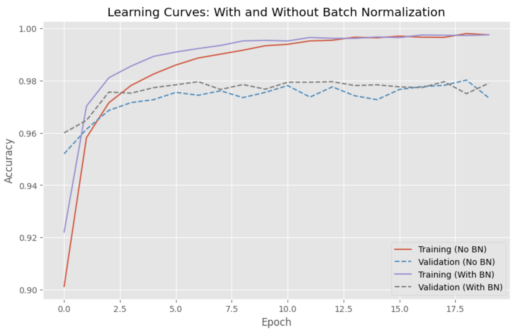
The learning curves show that the model with batch normalization converges more quickly and achieves a higher validation accuracy than the model without batch normalization.

References

https://towardsdatascience.com/batch-normalization-in-3-levels-of-understanding-14c2da90a338
http://static.googleusercontent.com/media/research.google.com/en//pubs/archive/43442.pdf
https://www.youtube.com/watch?v=yXOMHOpbon8&ab_channel=AssemblyAI