


What is a Convolutional Neural Network (CNN)
A Convolutional Neural Network (CNN) is a type of artificial neural network designed to process grid-like structured data, such as images, by using convolutional layers, pooling layers, and fully connected layers. CNNs have been widely used in computer vision tasks, including image classification, object detection, and semantic segmentation, among others.
Architecture of CNN
Input Layer
The input layer is the initial point of a CNN where raw data, such as images, are fed into the network. For images, the input is typically represented as a 3-dimensional tensor with height, width, and channels (e.g., red, green, and blue channels for color images). The input layer's primary role is to preprocess and standardize the input data to ensure that the network can effectively learn from it.
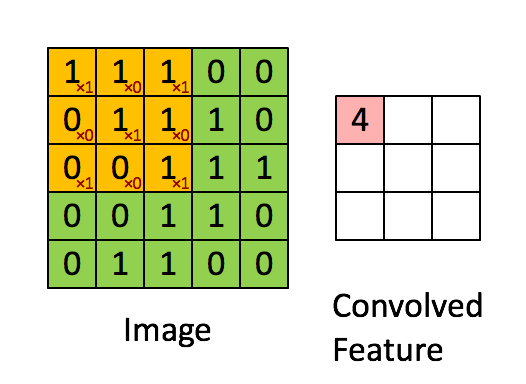
Convolutional Layer
The convolutional layer is the core component of a CNN. It applies a series of filters, also known as kernels, to the input data, which allows the network to learn local features such as edges, textures, and shapes. The filters are slid over the input data, performing element-wise multiplication and summing the results to produce feature maps. Each filter in the convolutional layer is responsible for detecting a specific feature in the input data.
Feature Maps
Feature maps are the outputs of the convolutional layer, which capture the presence of learned features in the input data. They are generated by applying filters or kernels to the input data using the convolution operation. As the CNN progresses through multiple layers, the feature maps become more abstract and higher-level, enabling the network to recognize complex patterns and structures.
A Comprehensive Guide to Convolutional Neural Networks — the ELI5 way
The pink matrix is the feature map.
Filters (Kernels)
Filters, also known as kernels, are small matrices used in the convolutional layer to extract features from the input data. Each filter is responsible for detecting a specific feature, such as an edge, texture, or shape. Filters are initialized with random values and are learned by the network during the training process. The size of the filters, known as the filter dimensions or kernel size, is a hyperparameter that can be adjusted to control the granularity of the learned features.
A Comprehensive Guide to Convolutional Neural Networks — the ELI5 way
The yellow matrix is the filter.
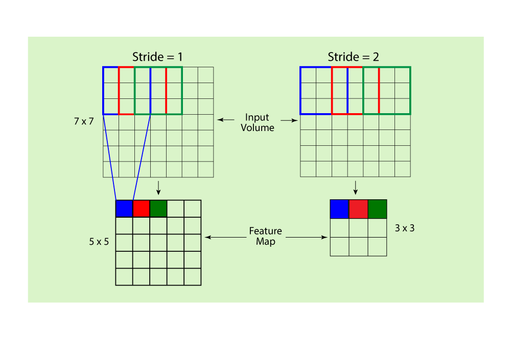
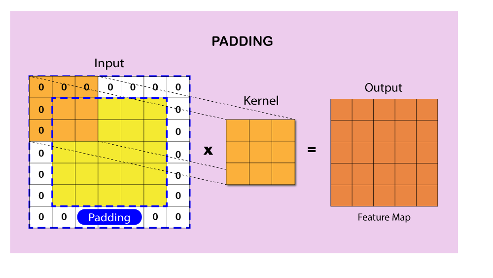
Stride and Padding
Stride and padding are hyperparameters that control the convolution operation in the convolutional layer. The stride is the number of pixels by which the filter is moved across the input data during the convolution. A larger stride results in a smaller feature map and reduces computational complexity. Padding refers to the process of adding extra pixels around the input data, typically with zero values, to maintain the spatial dimensions of the feature maps after the convolution operation. There are two main types of padding: 'valid' padding, where no padding is applied, and 'same' padding, where padding is added to ensure the output feature map has the same dimensions as the input data. Adjusting the stride and padding can have a significant impact on the performance and computational efficiency of a CNN.
Activation Functions
Activation functions are used to introduce non-linearity into the CNN, enabling it to learn complex patterns and representations. They are applied to the outputs of the convolutional layer, transforming the feature maps. Some popular activation functions used in CNNs include the Rectified Linear Unit (ReLU), Leaky ReLU, Sigmoid, and Hyperbolic Tangent (tanh). ReLU is the most commonly used activation function due to its computational efficiency and ability to mitigate the vanishing gradient problem.
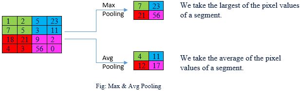
Pooling Layer
The pooling layer is responsible for downsampling the feature maps generated by the convolutional layer, reducing their spatial dimensions and computational complexity. This layer helps the network become more invariant to translation, rotation, and scaling, improving its ability to recognize features. There are various types of pooling operations, such as max pooling, average pooling, and global average pooling. Max pooling is the most widely used method, which selects the maximum value within a specified region in the feature map.
Convolutional Neural Network: An Overview
Fully Connected Layer (Affine Layer)
After several convolutional and pooling layers, the CNN often contains one or more fully connected layers. These layers are responsible for integrating the learned features from the previous layers and making high-level decisions based on the extracted patterns. Fully connected layers are similar to those found in traditional feedforward neural networks, where each neuron is connected to all neurons in the previous and subsequent layers.
Output Layer
The output layer is the final layer of a CNN and is responsible for producing the network's predictions or classifications. This layer typically uses the softmax activation function, which normalizes the outputs to generate a probability distribution over the possible classes. For regression tasks, the output layer may use a linear activation function instead. The loss function, such as cross-entropy or mean squared error, is then used to measure the difference between the network's predictions and the ground truth, guiding the optimization process during training.
Implementing CNNs using Python
In this section, I will implement a simple CNN using the PyTorch framework and train it on the public CIFAR-10 dataset. The CIFAR-10 dataset consists of 60,000 32x32 color images in 10 classes, with 6,000 images per class. There are 50,000 training images and 10,000 test images.
First, let's import the necessary libraries:
import torch
import torch.nn as nn
import torch.optim as optim
from torch.utils.data import DataLoader
import torchvision.transforms as transforms
import torchvision.datasets as datasets
Next, define the CNN architecture:
class SimpleCNN(nn.Module):
    def __init__(self):
        super(SimpleCNN, self).__init__()
        self.conv1 = nn.Conv2d(in_channels=3, out_channels=32, kernel_size=3, padding=1)
        self.relu1 = nn.ReLU()
        self.pool1 = nn.MaxPool2d(kernel_size=2, stride=2)
        self.conv2 = nn.Conv2d(in_channels=32, out_channels=64, kernel_size=3, padding=1)
        self.relu2 = nn.ReLU()
        self.pool2 = nn.MaxPool2d(kernel_size=2, stride=2)
        self.fc1 = nn.Linear(64 * 8 * 8, 128)
        self.relu3 = nn.ReLU()
        self.fc2 = nn.Linear(128, 10)

    def forward(self, x):
        x = self.pool1(self.relu1(self.conv1(x)))
        x = self.pool2(self.relu2(self.conv2(x)))
        x = x.view(x.size(0), -1)
        x = self.relu3(self.fc1(x))
        x = self.fc2(x)
        return x

model = SimpleCNN()
Now, define the loss function, optimizer, and other configurations:
criterion = nn.CrossEntropyLoss()
optimizer = optim.SGD(model.parameters(), lr=0.001, momentum=0.9)
device = torch.device("cuda:0" if torch.cuda.is_available() else "cpu")
model = model.to(device)
Load the CIFAR-10 dataset and apply data augmentation:
transform = transforms.Compose([
    transforms.RandomHorizontalFlip(),
    transforms.RandomCrop(32, padding=4),
    transforms.ToTensor(),
    transforms.Normalize((0.5, 0.5, 0.5), (0.5, 0.5, 0.5))
])

train_dataset = datasets.CIFAR10(root='./data', train=True, download=True, transform=transform)
test_dataset = datasets.CIFAR10(root='./data', train=False, download=True, transform=transform)

train_loader = DataLoader(train_dataset, batch_size=100, shuffle=True, num_workers=2)
test_loader = DataLoader(test_dataset, batch_size=100, shuffle=False, num_workers=2)
Train the model:
num_epochs = 10

for epoch in range(num_epochs):
    model.train()
    running_loss = 0.0

    for i, data in enumerate(train_loader, 0):
        inputs, labels = data
        inputs, labels = inputs.to(device), labels.to(device)

        optimizer.zero_grad()
        outputs = model(inputs)
        loss = criterion(outputs, labels)
        loss.backward()
        optimizer.step()

        running_loss += loss.item()

    print(f"Epoch {epoch + 1}, Loss: {running_loss / (i + 1)}")
Evaluate the model's performance on the test dataset:
model.eval()
correct = 0
total = 0

with torch.no_grad():
    for data in test_loader:
        inputs, labels = data
        inputs, labels = inputs.to(device), labels.to(device)

        outputs = model(inputs)
        _, predicted = torch.max(outputs.data, 1)

        total += labels.size(0)
        correct += (predicted == labels).sum().item()

print(f"Accuracy of the model on the 10,000 test images: {100 * correct / total}%")
Epoch 1, Loss: 2.1893566000461577
Epoch 2, Loss: 1.9117810306549072
Epoch 3, Loss: 1.7671691884994507
Epoch 4, Loss: 1.662340677499771
Epoch 5, Loss: 1.5774701907634736
Epoch 6, Loss: 1.5232401647567748
Epoch 7, Loss: 1.4739297952651977
Epoch 8, Loss: 1.431945639371872
Epoch 9, Loss: 1.39970556807518
Epoch 10, Loss: 1.3656729533672334
Accuracy of the model on the 10,000 test images: 51.57%
Visualizing What CNNs See
In this chapter, I will explore the inner workings of a CNN by visualizing what it "sees" as an input image passes through its layers. We will use images from a public dataset and PyTorch to create visualizations that help us understand the viewpoint of the CNN at different depths.
Let's import the necessary libraries and load the CIFAR-10 dataset:
import torch
import torchvision
import torchvision.transforms as transforms

# Data normalization
transform = transforms.Compose(
    [transforms.ToTensor(),
     transforms.Normalize((0.5, 0.5, 0.5), (0.5, 0.5, 0.5))])

# Load CIFAR-10 dataset
trainset = torchvision.datasets.CIFAR10(root='./data', train=True,
                                        download=True, transform=transform)
trainloader = torch.utils.data.DataLoader(trainset, batch_size=10,
                                          shuffle=True, num_workers=2)
Loading a Pre-trained CNN Model
For our visualization, we will use a pre-trained CNN model provided by PyTorch. We will use the VGG16 model, which is a popular and well-performing architecture. Load the pre-trained VGG16 model as follows:
import torchvision.models as models

# Load the pre-trained VGG16 model
vgg16 = models.vgg16(pretrained=True)
Visualizing the CNN's Viewpoint
To visualize what the CNN "sees" at different layers, we will create a function that extracts the feature maps from a given layer and plots them as images. The following code demonstrates how to do this using PyTorch and the matplotlib:
import matplotlib.pyplot as plt
import numpy as np

def visualize_layer(model, input_image, layer_index):
    # Define a forward hook to extract the output of the target layer
    def hook(module, input, output):
        global layer_output
        layer_output = output.detach()

    # Register the forward hook
    handle = model.features[layer_index].register_forward_hook(hook)

    # Run the input image through the model
    output = model(input_image.unsqueeze(0))

    # Remove the forward hook
    handle.remove()

    # Plot the feature maps
    num_feature_maps = layer_output.shape[1]
    rows = int(np.sqrt(num_feature_maps))
    cols = int(np.ceil(num_feature_maps / rows))

    fig, axes = plt.subplots(rows, cols, figsize=(cols*2, rows*2))

    for i in range(rows * cols):
        ax = axes[i // cols, i % cols]
        if i < num_feature_maps:
            ax.imshow(layer_output[0, i].numpy(), cmap='gray')
        ax.axis('off')

    plt.show()
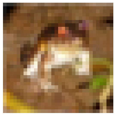
Let's select a sample image from the CIFAR-10 dataset and preprocess it:
sample_image, label = trainset[0]
sample_image = (sample_image * 0.5 + 0.5).permute(1, 2, 0).numpy()

# Plot the original image
plt.imshow(sample_image)
plt.axis('off')
plt.show()
Now, let's visualize the feature maps at different layers of the VGG16 model:
# Visualize the feature maps at layer 1 (first convolutional layer)
visualize_layer(vgg16, trainset[0][0], layer_index=0)

# Visualize the feature maps at layer 5 (fifth convolutional layer)
visualize_layer(vgg16, trainset[0][0], layer_index=4)

# Visualize the feature maps at layer 15 (fifteenth convolutional layer)
visualize_layer(vgg16, trainset[0][0], layer_index=14)
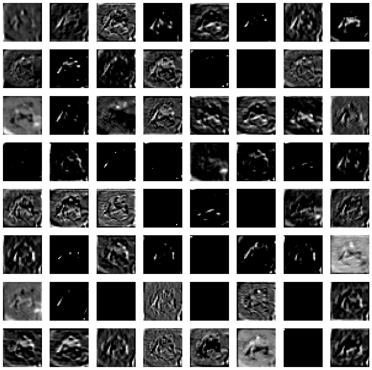
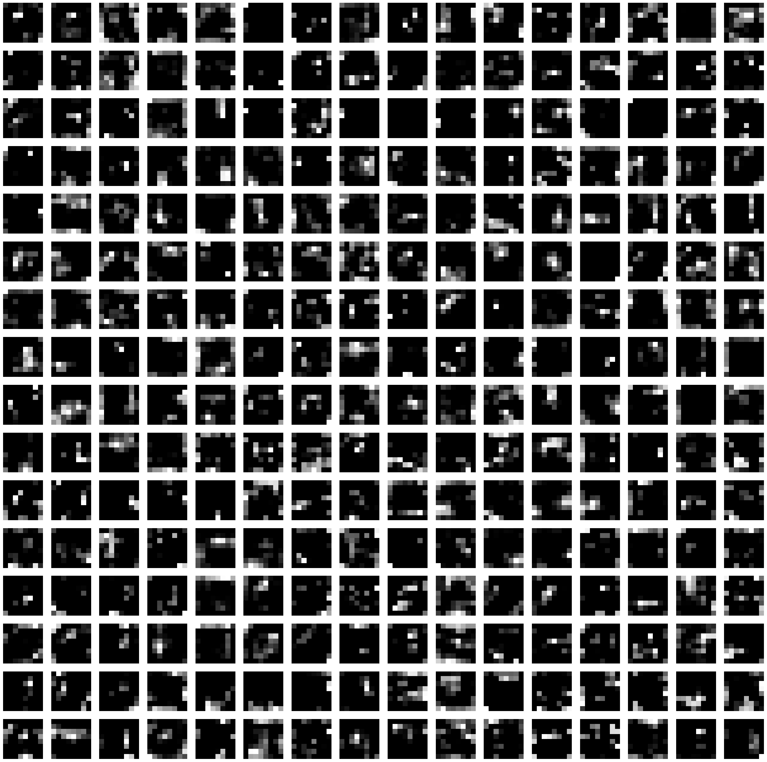
These visualizations show how the CNN "sees" the input image at different depths within the network. In the earlier layers, the feature maps capture simple patterns such as edges, corners, and textures. As the image progresses through the layers, the feature maps become more abstract and complex, representing higher-order patterns that help the CNN distinguish between different classes in the dataset.
References


Ryusei Kakujo


Weave the future of cities through data
Transportation modeling/ Urban planning/ Machine learning/ Computer science/ GIS