Introduction

The distribution of activations in hidden layers plays a crucial role in the learning process of neural networks. Well-distributed activations allow the network to learn more complex functions and generalize better to new, unseen data. By analyzing the distribution of activations within hidden layers, researchers and practitioners can diagnose potential issues, optimize performance, and improve the overall efficiency of a model.

Methods to Analyze Activation Distributions

To better understand the distribution of activations in hidden layers, various visualization and analysis techniques can be employed:

• Histograms
  A histogram is a common method to visualize activation distributions. By plotting the frequency of activations within specific value ranges, it provides insights into the shape and spread of the distribution, which can help identify issues like vanishing or exploding gradients.

• Density Plots
  Density plots provide a smoothed, continuous representation of the distribution of activations. This can help reveal the underlying structure of the distribution and identify potential areas of concern, such as dead neurons or a lack of diversity in activation values.

• Cumulative Distribution Function (CDF) Plots
  CDF plots visualize the cumulative probabilities of activation values. By analyzing the slope of the CDF plot, one can identify regions where activations are concentrated or sparse, which can inform strategies for improving the distribution.

Common Activation Distribution Issues

Certain issues in the distribution of activations can negatively impact the learning process of a neural network:

• Vanishing Gradient
  Vanishing gradient is a problem where the gradient values become too small, causing the network's weights to update very slowly or not at all. This issue can lead to poor performance and slow convergence. It often occurs when using activation functions with a limited range of output values, such as the sigmoid or hyperbolic tangent functions.

• Exploding Gradient
  Exploding gradient occurs when gradient values become too large, leading to instability in the learning process and potentially causing the model to diverge. This problem is more common in deep networks and can be mitigated by using proper weight initialization, gradient clipping, or normalization techniques.

• Dead Neurons
  Dead neurons refer to the situation where certain neurons in the hidden layers consistently output the same value, regardless of input. This can happen when using activation functions that have regions of zero gradient, such as the ReLU function. Dead neurons can hinder the learning process, as they do not contribute meaningfully to the network's output.

Optimizing Activation Distributions

To address the issues mentioned above and optimize the distribution of activations in hidden layers, several techniques can be applied:

• Selecting Appropriate Activation Functions
  Using activation functions that allow for a wider range of output values and gradients can help prevent vanishing or exploding gradients. For example, ReLU and its variants have gained popularity due to their ability to maintain non-zero gradients over a large input range.

• Adaptive Learning Rates
  Employing adaptive learning rate algorithms, such as Adam or RMSProp, can help mitigate the effects of vanishing or exploding gradients by adjusting the learning rate for each weight individually.

• Weight Initialization Techniques
  Proper weight initialization, such as Xavier or He initialization, can help prevent vanishing or exploding gradients by ensuring that the initial weights do not cause activations to become too small or too large.

  Regularization Techniques
  Applying regularization techniques, such as L1 or L2 regularization, can help mitigate the effects of dead neurons by encouraging sparsity or preventing weights from becoming too large.

• Normalization Techniques
  Normalization techniques, such as batch normalization or layer normalization, can help stabilize the learning process and improve the distribution of activations by normalizing the inputs to each hidden layer during training. This can lead to faster convergence and improved generalization.

• Gradient Clipping
  Gradient clipping is a technique that limits the magnitude of gradients during backpropagation. By preventing gradients from becoming too large, it can help mitigate the effects of exploding gradients and improve the stability of the learning process.

• Skip Connections
  Skip connections, as used in architectures like Residual Networks (ResNet), allow the gradients to flow more easily through the network by bypassing certain layers. This can help alleviate the vanishing gradient problem, especially in deeper networks.

Techniques for Better Activation Distributions

In this chapter, I delve deeper into various techniques that can be employed to improve the activation distributions in hidden layers, thereby enhancing the performance and efficiency of neural networks.

Weight Initialization

The initialization of weights in a neural network has a significant impact on the activation distributions. Proper weight initialization can prevent vanishing or exploding gradients and promote faster convergence. Some popular weight initialization methods are:

• Xavier (Glorot) Initialization
  This method sets the initial weights based on the size of the input and output units in the layer. It is particularly effective when used with sigmoid and hyperbolic tangent activation functions.

• He Initialization
  Similar to Xavier initialization, He initialization takes into account the size of the input and output units but is specifically designed for ReLU and its variants.

• LeCun Initialization
  This method is tailored for the sigmoid and hyperbolic tangent activation functions and considers only the size of the input units in the layer.

Batch Normalization

Batch normalization is a technique that normalizes the inputs to each hidden layer during training by scaling and shifting the activations. It helps stabilize the learning process, speeds up convergence, and improves the generalization performance of the network. Batch normalization can be particularly useful in addressing vanishing or exploding gradients and promoting more evenly distributed activations.

Layer Normalization

Layer normalization is an alternative to batch normalization, particularly useful when dealing with variable-length sequences or small batch sizes. Instead of normalizing the inputs across the batch, layer normalization normalizes the inputs across the features within each hidden layer. This can lead to more stable activation distributions and improved learning dynamics.

Regularization

Regularization techniques can help improve activation distributions by encouraging sparsity or preventing weights from becoming too large. Some common regularization methods are:

• L1 Regularization
  L1 regularization adds an L1 penalty, proportional to the absolute value of the weights, to the loss function. This encourages sparsity in the weight matrix, which can help mitigate the effects of dead neurons.

• L2 Regularization
  L2 regularization adds an L2 penalty, proportional to the square of the weights, to the loss function. This prevents weights from becoming too large and can help alleviate issues related to vanishing or exploding gradients.

• Dropout
  Dropout is a regularization technique where a random subset of neurons is "dropped out" or temporarily deactivated during training. This prevents the model from relying too heavily on any single neuron and encourages more evenly distributed activations.

Visualizing Activation Distribution in Hidden Layers

In this chapter, I will demonstrate how to visualize the activation distributions in hidden layers using the Iris dataset, which is a public dataset that contains 150 samples of iris flowers. We will train a simple feed-forward neural network (FFNN) on this dataset, draw histograms of the activations.

Dataset and Model Overview

The Iris dataset consists of 150 samples, with 50 samples from each of the three species of iris flowers (Iris setosa, Iris versicolor, and Iris virginica). Each sample has four features (sepal length, sepal width, petal length, and petal width) and a label indicating the species.

Our FFNN model will have the following architecture:

1. Input layer with 4 input nodes.
2. Fully connected (dense) layer with 64 units and ReLU activation.
3. Fully connected (dense) layer with 32 units and ReLU activation.
4. Fully connected (dense) layer with 16 units and ReLU activation.
5. Output layer with 3 units and softmax activation.

Preprocessing and Training

We will preprocess the data and train the model using the following Python code with PyTorch:

import torch
import torch.nn as nn
import torch.optim as optim
from torch.autograd import Variable
import torch.nn.functional as F
from sklearn import datasets
from sklearn.model_selection import train_test_split
from sklearn.preprocessing import StandardScaler
from sklearn.preprocessing import OneHotEncoder

# Load and preprocess the data
iris = datasets.load_iris()
X = iris.data
y = iris.target

# Normalize the features
scaler = StandardScaler()
X_scaled = scaler.fit_transform(X)

# One-hot encode the target labels
encoder = OneHotEncoder()
y_onehot = encoder.fit_transform(y.reshape(-1, 1)).toarray()

# Split the data into training and testing sets
X_train, X_test, y_train, y_test = train_test_split(
    X_scaled, y_onehot, test_size=0.2, random_state=42)

# Convert the data to PyTorch tensors
X_train = Variable(torch.Tensor(X_train).float())
X_test = Variable(torch.Tensor(X_test).float())
y_train = Variable(torch.Tensor(y_train).float())
y_test = Variable(torch.Tensor(y_test).float())

# Define the model
class Iris_FFNN(nn.Module):
    def __init__(self):
        super(Iris_FFNN, self).__init__()
        self.fc1 = nn.Linear(4, 64)
        self.fc2 = nn.Linear(64, 32)
        self.fc3 = nn.Linear(32, 16)
        self.fc4 = nn.Linear(16, 3)

    def forward(self, x):
        x = F.relu(self.fc1(x))
        x = F.relu(self.fc2(x))
        x = F.relu(self.fc3(x))
        x = self.fc4(x)
        return x

model = Iris_FFNN()

# Set loss function and optimizer
criterion = nn.MSELoss()
optimizer = optim.Adam(model.parameters(), lr=0.001)

# Train the model
num_epochs = 500
for epoch in range(num_epochs):
    optimizer.zero_grad()
    outputs = model(X_train)
    loss = criterion(outputs, y_train)
    loss.backward()
    optimizer.step()
    if (epoch + 1) % 50 == 0:
        print(f'Epoch [{epoch+1}/{num_epochs}], Loss: {loss.item()}')

print('Finished training')

Visualizing Activation Distributions

To visualize the activation distributions in the hidden layers, we will draw histograms of the activations for layers 1, 2, and 3. To do this, we will first create a function to extract the activations from the hidden layers:

def get_activations(model, layer_indices, input_data):
    activations = []

    for index in layer_indices:
        activation_model = nn.Sequential(*(list(model.children())[:index+1]))
        activation = activation_model(input_data)
        activations.append(activation)

    return activations

Next, we will pass a batch of test samples through the trained model and collect the activations from the hidden layers:

# Get the activations from the hidden layers
hidden_layer_indices = [0, 1, 2]
activations = get_activations(model, hidden_layer_indices, X_test)

Now, we will plot histograms of these activations using Matplotlib:

import matplotlib.pyplot as plt

plt.style.use('ggplot')

def plot_activation_histograms(activations, layer_indices):
    num_layers = len(activations)

    fig, axes = plt.subplots(1, num_layers, figsize=(15, 5))

    for i, activation in enumerate(activations):
        layer_index = layer_indices[i]
        axes[i].hist(activation.detach().numpy().flatten(), bins=50, orientation='vertical', alpha=0.5)
        axes[i].set_title(f'Layer {layer_index + 1} Activations')
        axes[i].set_xlabel('Activation Value')

    axes[0].set_ylabel('Frequency')
    plt.tight_layout()
    plt.show()

plot_activation_histograms(activations, hidden_layer_indices)

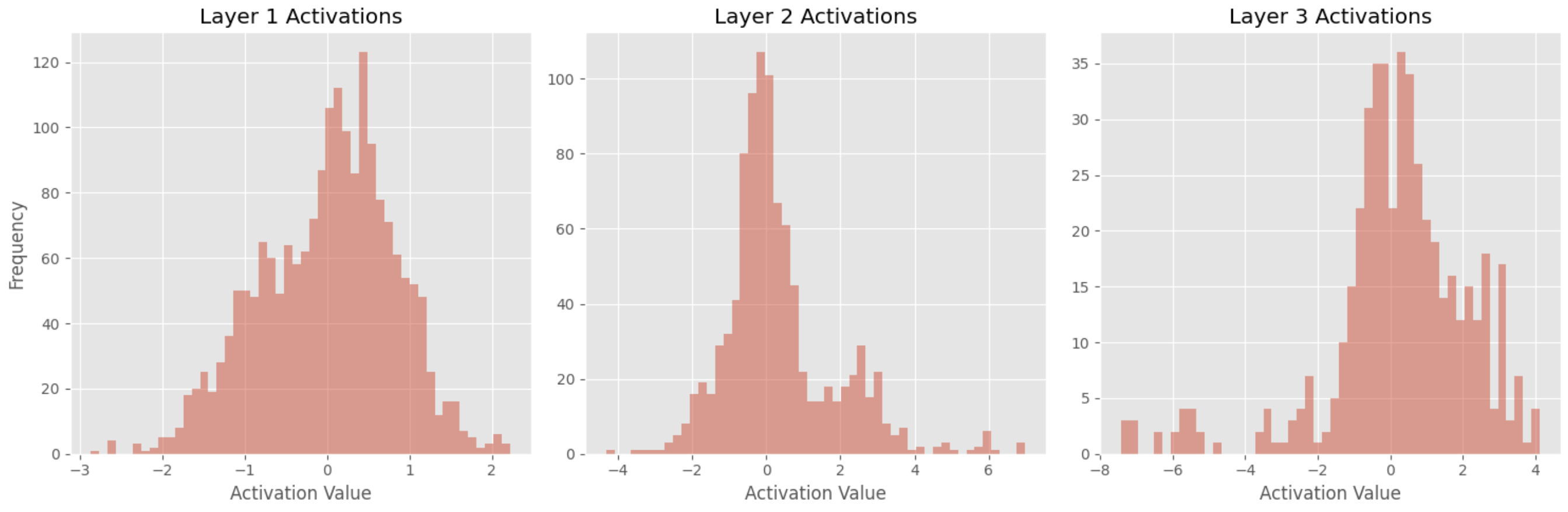
Interpreting the Results

After plotting the histograms, we can analyze the activation distributions and draw some conclusions:

• Most frequent value is 0
  The fact that the most frequent activation value is 0 across all 3 layers suggests that a large proportion of the neurons in the network are not being activated by the input data. This could be because the network is using ReLU activation function, which outputs 0 for all negative input values.

• Keen Kurtosis
  An increase in kurtosis from layer 1 to layer 3 suggests that the distribution of activation values becomes more peaked and has heavier tails as you move deeper into the neural network. This could indicate that the neurons in the deeper layers are selectively responding to specific features in the input data and ignoring others, which could be a sign of the network learning more complex representations of the data.

• Wider Range
  The widening of the range of activation values from layer 1 to layer 3 suggests that the neurons in the deeper layers are more sensitive to variations in the input data. This could be a sign of the network learning to extract more fine-grained features from the data.