2022-11-23

Polynomial Regression

Machine Learning

Regression

Python

sklearn

What is Polynomial Regression

Polynomial Regression is a form of regression analysis in which the relationship between the independent variable(s) and the dependent variable is modeled as an nth degree polynomial function. In simpler terms, it is an extension of linear regression that enables us to capture more complex, nonlinear relationships between variables. Polynomial Regression provides a flexible and powerful approach to modeling data with curved trends, oscillations, or other complex patterns.

Why Use Polynomial Regression

While linear regression models are easy to interpret and implement, they are limited in their ability to capture complex relationships between variables. In many real-world applications, the relationship between the input and output variables is not linear, and a straight line may not be the best representation of the underlying patterns in the data.

Polynomial Regression allows us to fit a curve to the data, enabling us to model a wider range of relationships between variables. Some key advantages of using Polynomial Regression include:

Flexibility
: By adjusting the degree of the polynomial, we can control the complexity of the model, allowing us to capture various patterns in the data.
Interpretability
Polynomial Regression models, while more complex than linear models, are still relatively easy to interpret and understand.
Applicability
Polynomial Regression can be applied to a wide range of problems, from predicting housing prices to modeling the spread of infectious diseases.

Mathematics Behind Polynomial Regression

Linear Regression: A Foundation

Linear regression is the simplest form of regression analysis, where the relationship between the independent variable $x$ and the dependent variable $y$ is modeled as a linear function. The equation for a linear regression model can be represented as:

$y = \beta_0 + \beta_1x + \epsilon$

where $y$ is the dependent variable, $x$ is the independent variable, $\beta_0$ is the intercept, $\beta_1$ is the slope of the line, and $\epsilon$ is the error term.

Polynomial Functions

Polynomial functions are mathematical expressions that consist of variables and coefficients, involving only the operations of addition, subtraction, multiplication, and non-negative integer exponents. A polynomial of degree $n$ can be represented as:

$P(x) = a_0 + a_1x + a_2x^2 + \cdots + a_nx^n$

where $a_i$ are the coefficients and $x$ is the variable.

Polynomial Regression Model

In polynomial regression, we extend the linear regression model by fitting a polynomial function to the data. For a univariate polynomial regression of degree $n$ , the equation can be represented as:

$y = \beta_0 + \beta_1x + \beta_2x^2 + \cdots + \beta_nx^n + \epsilon$

The goal of polynomial regression is to find the coefficients $\beta_i$ that best fit the data, minimizing the error term $\epsilon$ .

Finding the Coefficients: Least Squares Method

The Least Squares Method is an optimization technique used to find the best-fitting coefficients for a polynomial regression model. The objective is to minimize the sum of the squared residuals (the difference between the observed values and the predicted values), also known as the residual sum of squares (RSS).

$RSS(\beta) = \sum_{i=1}^{N} [y_i - (\beta_0 + \beta_1x_i + \beta_2x_i^2 + \cdots + \beta_nx_i^n)]^2$

To find the coefficients that minimize the RSS, we can take the partial derivatives of the RSS function with respect to each coefficient and set them equal to zero. Solving this system of linear equations will yield the optimal values for the coefficients $\beta_i$ .

Implementing Polynomial Regression in Python

In this chapter, I will demonstrate how to implement polynomial regression using Python, focusing on the popular "mpg" dataset.

First, we will import the necessary libraries and load the "mpg" dataset. The dataset is available in the seaborn library.

python

import numpy as np
import pandas as pd
import seaborn as sns
import matplotlib.pyplot as plt
from sklearn.model_selection import train_test_split
from sklearn.preprocessing import PolynomialFeatures
from sklearn.linear_model import LinearRegression
from sklearn.metrics import mean_squared_error, r2_score

# Load the mpg dataset
mpg = sns.load_dataset("mpg")

# Display the first five rows
print(mpg.head())

    mpg  cylinders  displacement  horsepower  weight  acceleration  \
0  18.0          8         307.0       130.0    3504          12.0
1  15.0          8         350.0       165.0    3693          11.5
2  18.0          8         318.0       150.0    3436          11.0
3  16.0          8         304.0       150.0    3433          12.0
4  17.0          8         302.0       140.0    3449          10.5

   model_year origin                       name
0          70    usa  chevrolet chevelle malibu
1          70    usa          buick skylark 320
2          70    usa         plymouth satellite
3          70    usa              amc rebel sst
4          70    usa                ford torino

For this example, we will use the horsepower feature as the independent variable (x) and mpg as the dependent variable (y). We will also remove any rows with missing values.

python

# Remove missing values and select the relevant columns
mpg_cleaned = mpg[['horsepower', 'mpg']].dropna()

# Separate the features and the target variable
X = mpg_cleaned['horsepower'].values.reshape(-1, 1)
y = mpg_cleaned['mpg'].values

Now we will create polynomial features for our independent variable horsepower. For this example, we will use a polynomial of degree 2.

python

# Create polynomial features
poly_features = PolynomialFeatures(degree=2)
X_poly = poly_features.fit_transform(X)

We will split the data into training and testing sets, train our polynomial regression model, and evaluate its performance using mean squared error (MSE) and R-squared.

python

# Split the data into training and testing sets
X_train, X_test, y_train, y_test = train_test_split(X_poly, y, test_size=0.2, random_state=42)

# Train the polynomial regression model
poly_reg = LinearRegression()
poly_reg.fit(X_train, y_train)

# Make predictions and evaluate the model
y_pred = poly_reg.predict(X_test)
mse = mean_squared_error(y_test, y_pred)
r2 = r2_score(y_test, y_pred)

print("Mean Squared Error: ", round(mse, 2))
print("R-squared: ", round(r2, 2))

Mean Squared Error:  18.42
R-squared:  0.64

Finally, we will visualize the polynomial regression using matplotlib and seaborn.

python

# Set seaborn style
sns.set(style="whitegrid")

# Create a scatterplot of the data
plt.figure(figsize=(10, 6))
plt.scatter(X, y, color='blue', alpha=0.5, label="Data points")

# Plot the polynomial regression curve
X_plot = np.linspace(X.min(), X.max(), 100).reshape(-1, 1)
X_plot_poly = poly_features.transform(X_plot)
y_plot = poly_reg.predict(X_plot_poly)
plt.plot(X_plot, y_plot, color='red', linewidth=2, label="Polynomial Regression")

# Customize the plot appearance
plt.xlabel("Horsepower")
plt.ylabel("Miles per Gallon (mpg)")
plt.title("Polynomial Regression of Degree 2: Horsepower vs. MPG")
plt.legend()
plt.show()

Polynomial regression

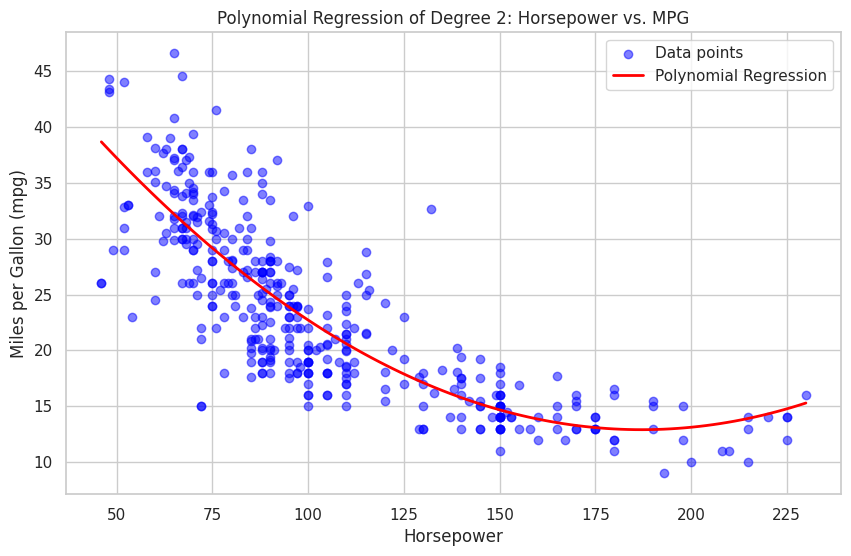
The resulting plot displays the polynomial regression, highlighting the relationship between horsepower and mpg. You can experiment with different degrees of the polynomial or other features in the dataset to explore how the model's performance and visualization change.