2022-11-24

Support Vector Regression

Machine Learning

Regression

Python

sklearn

What is Support Vector Regression (SVR)

Support Vector Regression (SVR) is a powerful and versatile machine learning algorithm derived from the well-known Support Vector Machines (SVM) for classification. The primary goal of SVR is to predict a continuous target variable, given a set of input features.

Key Concepts in SVR

SVR aims to find a function that approximates the relationship between input features and the target variable, with the objective of minimizing the prediction error within a specified tolerance margin. The main concepts in SVR include:

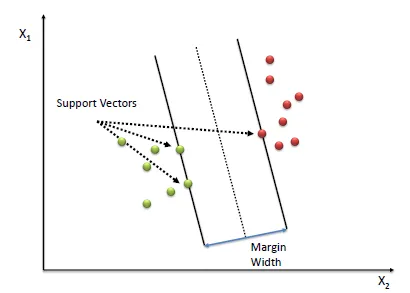
Support vectors
These are the data points that lie on or outside the specified margin around the approximating function. Support vectors play a crucial role in defining the SVR model, as they determine the optimal parameters.

Machine Learning: Support Vector Regression (SVR)

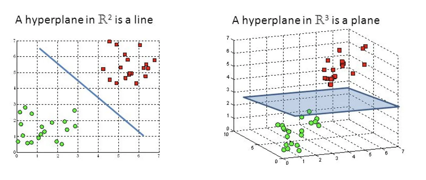
Hyperplane
A hyperplane is a flat subspace of one dimension less than the ambient space. In the context of SVR, the hyperplane is used to approximate the relationship between input features and the target variable. For linear SVR, the hyperplane represents a linear function, while for nonlinear SVR, the hyperplane exists in a higher-dimensional space obtained through kernel transformation.

Hyperplane
Machine Learning: Support Vector Regression (SVR)

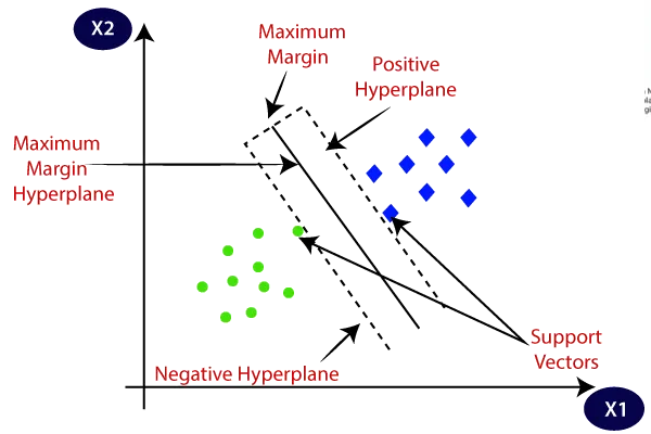
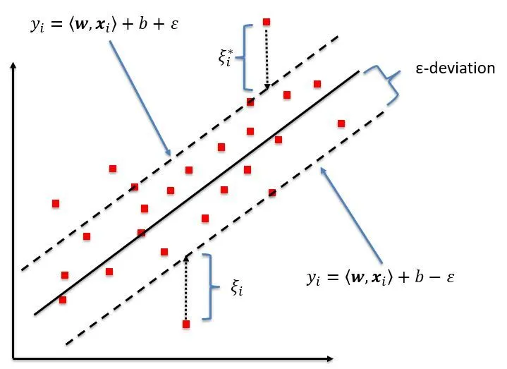
Margin
The margin is a tolerance zone around the approximating function (hyperplane) within which errors are considered acceptable. SVR aims to maximize the margin while keeping the prediction error within the specified tolerance. The width of the margin is determined by the parameter $\epsilon$ .

Margin
Machine Learning: Support Vector Regression (SVR)

SVR
Machine Learning: Support Vector Regression (SVR)

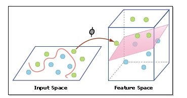
Kernel Trick
The kernel trick is a technique used in nonlinear SVR to find a nonlinear function that best approximates the relationship between input features and the target variable, while keeping the prediction error within the specified tolerance margin. The kernel trick involves mapping the input data to a higher-dimensional space using a kernel function, where a linear function can be used to approximate the nonlinear relationship. This allows SVR to solve nonlinear problems without explicitly transforming the input data, thus reducing computational complexity.

kernel
Support Vector Regression Tutorial for Machine Learning

Mathematical Foundations of SVR

Linear Regression vs. SVR

In linear regression, we try to find the best-fitting line by minimizing the squared error between the predicted values and the actual values. The linear function is given by:

f(x) = w^T x + b

Where $w$ is the weight vector, $x$ is the input feature vector, and $b$ is the bias term. In contrast, SVR focuses on finding a function that lies within a specified margin (tolerance) around the true target values.

Optimization Problem

SVR aims to find the optimal weight vector $w$ and bias term $b$ by solving the following optimization problem:

Objective Function

\min_{w, b} \frac{1}{2} ||w||^2 + C \sum_{i=1}^N (\xi_i + \xi_i^*)

Where $||w||^2$ is the squared norm of the weight vector $w$ , $C$ is the regularization parameter, $N$ is the number of data points, and $\xi_i$ and $\xi_i^*$ are slack variables that measure the deviation of predictions from the true target values.

Constraints

The constraints for the optimization problem are defined as follows:

\begin{aligned} y_i - f(x_i) &\leq \epsilon + \xi_i \\ f(x_i) - y_i &\leq \epsilon + \xi_i^* \\ \xi_i, \xi_i^* &\geq 0, \quad i = 1, \dots, N \end{aligned}

Where $y_i$ is the true target value for the $i$ -th data point, and $\epsilon$ is the tolerance margin.

Loss Functions

SVR uses the $\epsilon$ -insensitive loss function, which is defined as follows:

L_\epsilon(y, f(x)) = \max(0, |y - f(x)| - \epsilon)

The $\epsilon$ -insensitive loss function does not penalize errors that lie within the specified margin $\epsilon$ .

Dual Formulation

The dual formulation of the SVR problem is obtained by applying the Karush-Kuhn-Tucker (KKT) conditions to the Lagrangian function. This reformulation allows us to solve the optimization problem more efficiently and to incorporate nonlinear kernels.

Lagrange Multipliers

To derive the dual problem, we introduce Lagrange multipliers $\alpha_i, \alpha_i^* \geq 0$ for each constraint in the optimization problem. The Lagrangian function is then defined as:

\mathcal{L}(w, b, \xi, \xi^*, \alpha, \alpha^*) = \frac{1}{2} ||w||^2 + C \sum_{i=1}^N (\xi_i + \xi_i^*) - \sum_{i=1}^N (\alpha_i - \alpha_i^*)(y_i - w^T x_i - b - \epsilon - \xi_i) - \sum_{i=1}^N (\alpha_i + \alpha_i^*)(\xi_i + \xi_i^*)

Karush-Kuhn-Tucker (KKT) Conditions

Applying the KKT conditions to the Lagrangian function results in the dual problem, which involves maximizing the following dual objective function with respect to the Lagrange multipliers $\alpha$ and $\alpha^*$ :

\max_{\alpha, \alpha^*} \Bigg( -\frac{1}{2} \sum_{i=1}^N \sum_{j=1}^N (\alpha_i - \alpha_i^*)(\alpha_j - \alpha_j^*) y_i y_j x_i^T x_j + \sum_{i=1}^N (\alpha_i + \alpha_i^*) y_i - \epsilon \sum_{i=1}^N (\alpha_i + \alpha_i^*) \Bigg)

Subject to the following constraints:

\begin{aligned} \sum_{i=1}^N (\alpha_i - \alpha_i^*) &= 0 \\ \alpha_i, \alpha_i^* &\in [0, C], \quad i = 1, \dots, N \end{aligned}

The dual formulation enables us to solve the SVR problem more efficiently, especially when using nonlinear kernels. By replacing the inner product $x_i^T x_j$ with the kernel function $K(x_i, x_j)$ in the dual objective function, we can efficiently handle nonlinear relationships without explicitly transforming the input data.

Kernel Trick

Kernel Functions

In nonlinear SVR, we use the kernel trick to map the input data to a higher-dimensional space, where a linear function can be used to approximate the nonlinear relationship. A kernel function is a similarity measure that computes the inner product between two input feature vectors in the transformed space:

K(x_i, x_j) = \phi(x_i)^T \phi(x_j)

Where $\phi(x_i)$ and $\phi(x_j)$ are the mappings of input feature vectors $x_i$ and $x_j$ to the transformed space.

Popular Kernels in SVR

Some popular kernel functions used in SVR include:

Linear kernel

K(x_i, x_j) = x_i^T x_j

Polynomial kernel

K(x_i, x_j) = (x_i^T x_j + c)^d

Radial basis function (RBF) kernel

K(x_i, x_j) = \exp(-\gamma ||x_i - x_j||^2)

Sigmoid kernel

K(x_i, x_j) = \tanh(\kappa x_i^T x_j + c)

By replacing the inner product $x_i^T x_j$ with the kernel function $K(x_i, x_j)$ in the dual objective function, we obtain the dual problem for nonlinear SVR.

Implementing SVR in Python

In this chapter, I will implement SVR using Python and the scikit-learn library. We will use the Iris dataset and visualize the support vectors with various kernel functions.

First, let's load the Iris dataset and prepare it for regression.

python

from sklearn import datasets
from sklearn.model_selection import train_test_split

iris = datasets.load_iris()
X = iris.data[:, :2]  # Use the first two features.
y = iris.data[:, 2]   # Use the third feature as the target.

# Split the dataset into a training set and a test set.
X_train, X_test, y_train, y_test = train_test_split(X, y, test_size=0.3, random_state=42)

Now let's train the SVR model with various kernel functions.

python

from sklearn.svm import SVR

# Initialize SVR models with different kernels.
svr_linear = SVR(kernel='linear', C=1)
svr_poly = SVR(kernel='poly', C=1, degree=3)
svr_rbf = SVR(kernel='rbf', C=1, gamma='auto')

# Train the SVR models.
svr_linear.fit(X_train, y_train)
svr_poly.fit(X_train, y_train)
svr_rbf.fit(X_train, y_train)

To visualize the support vectors, we'll create a scatter plot of the data points and highlight the support vectors.

python

import matplotlib.pyplot as plt
import seaborn as sns
import numpy as np

sns.set(style="darkgrid")

def plot_support_vectors(svr_model, X, y, title, ax):
    h = .02  # step size in the mesh
    # Create a mesh to plot in.
    x_min, x_max = X[:, 0].min() - 1, X[:, 0].max() + 1
    y_min, y_max = X[:, 1].min() - 1, X[:, 1].max() + 1
    xx, yy = np.meshgrid(np.arange(x_min, x_max, h),
                         np.arange(y_min, y_max, h))

    # Predict target values for the mesh.
    Z = svr_model.predict(np.c_[xx.ravel(), yy.ravel()])
    Z = Z.reshape(xx.shape)

    # Plot the contour of the predictions.
    ax.contourf(xx, yy, Z, alpha=0.8)
    scatter = ax.scatter(X[:, 0], X[:, 1], c=y, edgecolors='k', marker='o', s=50)
    ax.set_title(title)
    ax.legend(*scatter.legend_elements())

fig, axes = plt.subplots(1, 3, figsize=(18, 6))
plot_support_vectors(svr_linear, X_train, y_train, 'SVR with Linear Kernel', axes[0])
plot_support_vectors(svr_poly, X_train, y_train, 'SVR with Polynomial Kernel', axes[1])
plot_support_vectors(svr_rbf, X_train, y_train, 'SVR with RBF Kernel', axes[2])

plt.show()

SVR with various kernel function

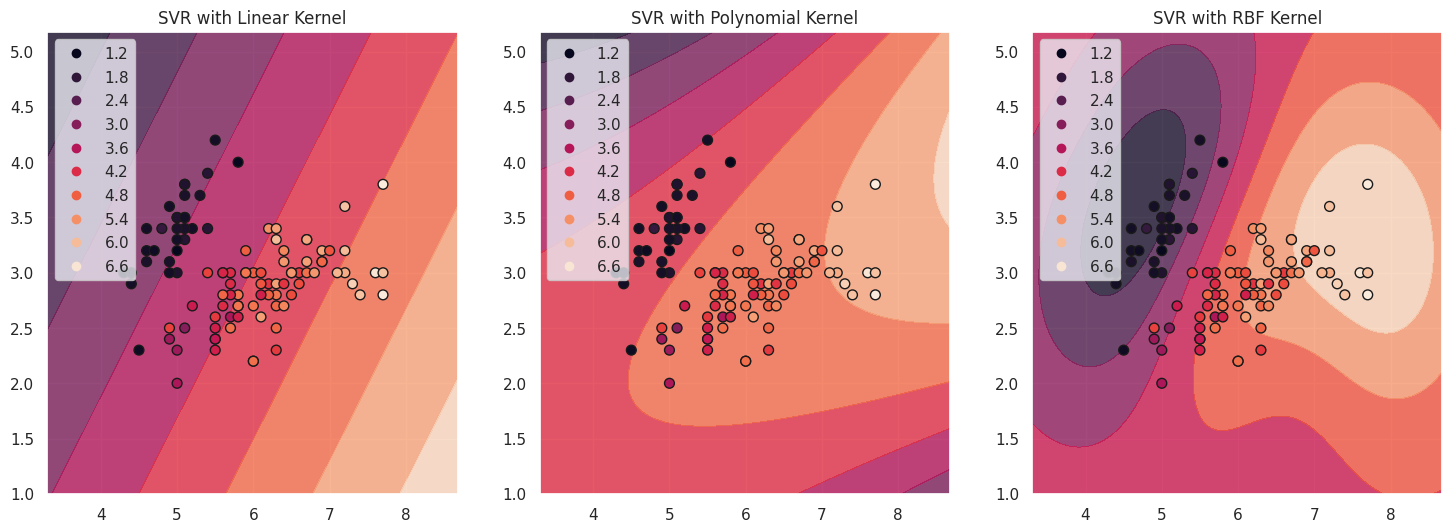
The support vectors are the data points that lie within or on the boundary of the margin. They are critical in determining the position of the hyperplane and have a significant influence on the model's predictions. In the plots above, the support vectors are represented by the points on the contour lines of the approximating functions for each kernel. These points play a key role in determining the shape of the decision boundary and the overall performance of the SVR model.

To evaluate the performance of our SVR models with different kernels, we can calculate their mean squared error (MSE) and R-squared scores on the test set.

python

from sklearn.metrics import mean_squared_error, r2_score

def evaluate_model(svr_model, X_test, y_test):
    y_pred = svr_model.predict(X_test)
    mse = mean_squared_error(y_test, y_pred)
    r2 = r2_score(y_test, y_pred)
    return mse, r2

mse_linear, r2_linear = evaluate_model(svr_linear, X_test, y_test)
mse_poly, r2_poly = evaluate_model(svr_poly, X_test, y_test)
mse_rbf, r2_rbf = evaluate_model(svr_rbf, X_test, y_test)

print("Linear kernel: MSE = {:.2f}, R^2 = {:.2f}".format(mse_linear, r2_linear))
print("Polynomial kernel: MSE = {:.2f}, R^2 = {:.2f}".format(mse_poly, r2_poly))
print("RBF kernel: MSE = {:.2f}, R^2 = {:.2f}".format(mse_rbf, r2_rbf))

Linear kernel: MSE = 0.31, R^2 = 0.91
Polynomial kernel: MSE = 0.54, R^2 = 0.84
RBF kernel: MSE = 0.30, R^2 = 0.91

This will output the mean squared error and R-squared scores for each of the SVR models. By comparing these metrics, we can determine which kernel provides the best fit for our data.