What is Support Vector Machine (SVM)

Support Vector Machine (SVM) is a powerful machine learning algorithm used for classification. SVM is a non-probabilistic binary linear classifier that tries to find the best hyperplane in the feature space that separates the data points of different classes with maximum margin. The hyperplane is chosen in such a way that it optimally separates the data points, and the margin is defined as the distance between the hyperplane and the closest data points from each class.

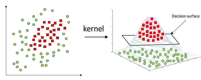
In addition to linearly separable data, SVM can also handle non-linearly separable data by using the kernel trick. The kernel trick involves mapping the input data into a higher-dimensional feature space where it can be linearly separated. SVM tries to find the optimal hyperplane in this higher-dimensional feature space to separate the data points.

Basic Concepts and Terminology

• Hyperplane
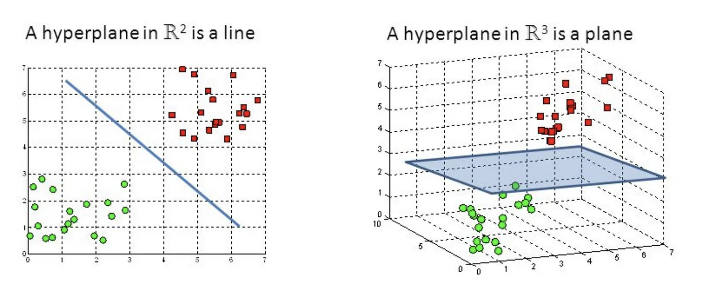
  A hyperplane is a geometrical object that generalizes the concept of a straight line (in 2D) or a plane (in 3D) to higher-dimensional spaces. In an n-dimensional space, a hyperplane is defined as an (n-1)-dimensional object.

Support Vector Machine — Introduction to Machine Learning Algorithms

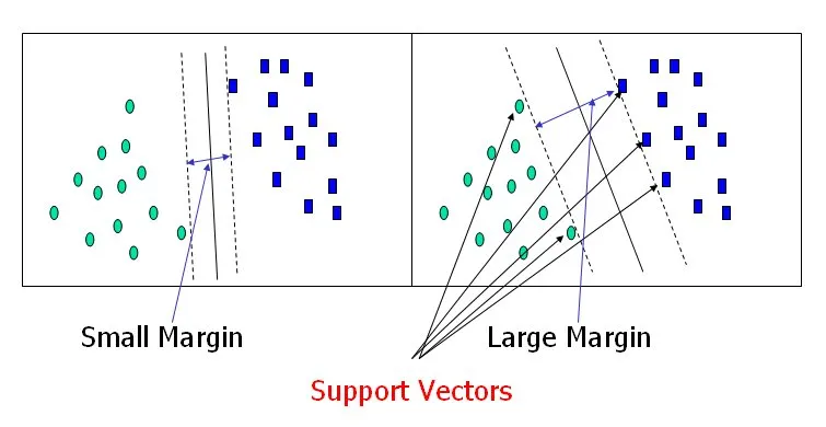
• Margin
  The margin is the distance between the separating hyperplane and the closest data points from different classes. The objective of SVM is to find a hyperplane that maximizes this margin, providing better generalization capabilities.

• Support Vectors
  Support vectors are the data points that lie closest to the separating hyperplane and contribute to defining the margin. These data points are critical in determining the position of the hyperplane.

Support Vector Machine — Introduction to Machine Learning Algorithms

• Linear Separability
  A dataset is said to be linearly separable if there exists a hyperplane that can perfectly separate the data points of different classes.

• Kernel Function
  A kernel function is a mathematical function that maps the original data points into a higher-dimensional feature space, enabling the SVM algorithm to handle non-linearly separable data.

  
  What is the kernel trick? Why is it important?

Mathematics Behind SVM

Linear Separability and Hyperplanes

Given a dataset with n-dimensional feature vectors, a hyperplane is defined as an (n-1)-dimensional object that can be represented by the equation:

where \boldsymbol{w} is the weight vector, \boldsymbol{x} is the feature vector, and b is the bias term. The goal of SVM is to find the optimal hyperplane that separates the data points of different classes.

Maximization of the Margin

The margin (M) is the distance between the hyperplane and the closest data points (support vectors) of different classes. For a given data point \boldsymbol{x}_i with class label y_i \in {-1, 1}, the equation of the hyperplane can be written as:

The distance from a data point \boldsymbol{x}_i to the hyperplane is given by:

Since we are interested in the margin, which is the smallest distance between the hyperplane and the data points of different classes, we have:

The objective of SVM is to maximize the margin M while maintaining the classification constraints:

Maximizing the margin M is equivalent to minimizing the squared Euclidean norm of the weight vector ||\boldsymbol{w}||^2.

Dual Problem and Lagrange Multipliers

To solve the constrained optimization problem, we can use Lagrange multipliers. The Lagrangian for the SVM optimization problem can be written as:

where N is the number of data points, and \boldsymbol{\alpha} is a vector of Lagrange multipliers.

We need to minimize \mathcal{L}(\boldsymbol{w}, b, \boldsymbol{\alpha}) with respect to \boldsymbol{w} and b and maximize it with respect to \boldsymbol{\alpha}. The saddle point conditions yield:

and

Substituting these conditions into the Lagrangian, we get the dual optimization problem:

subject to the constraints:

and

This dual problem is a quadratic programming problem, which can be solved using various optimization techniques such as the Sequential Minimal Optimization (SMO) algorithm or gradient-based methods.

Kernel Trick

In cases where the data is not linearly separable, SVM uses the kernel trick to transform the data into a higher-dimensional space where it becomes linearly separable. A kernel function K(\boldsymbol{x}_i, \boldsymbol{x}_j) is used to map the original data points into a new feature space, allowing the SVM algorithm to find an optimal separating hyperplane. The dual problem now becomes:

subject to the same constraints as before. Some popular kernel functions include the linear kernel, polynomial kernel, radial basis function (RBF) kernel, and the sigmoid kernel.

After solving the dual problem, the weight vector \boldsymbol{w} can be computed as:

where \phi(\boldsymbol{x}_i) is the mapped feature vector in the higher-dimensional space. The bias term b can be computed using any support vector \boldsymbol{x}_s:

The decision function for a new data point \boldsymbol{x}^* is then given by:

The kernel trick allows SVM to handle non−linearly separable data and provides a flexible way to incorporate domain knowledge into the algorithm by choosing an appropriate kernel function.

Implementing SVM with the Iris Dataset

In this chapter, I will implement SVM using Python and scikit-learn. We will use the Iris dataset to illustrate the classification capabilities of SVM with various kernels.

First, let's import the necessary libraries and load the Iris dataset:

import numpy as np
import matplotlib.pyplot as plt
import seaborn as sns
from sklearn import datasets
from sklearn.model_selection import train_test_split
from sklearn.svm import SVC
from sklearn.metrics import accuracy_score, classification_report, confusion_matrix

# Load the Iris dataset
iris = datasets.load_iris()
X = iris.data[:, :2]  # We will only use the first two features for visualization purposes
y = iris.target

We will split the dataset into training and testing sets, and train the SVM model with various kernels:

# Split the dataset into training and testing sets
X_train, X_test, y_train, y_test = train_test_split(X, y, test_size=0.3, random_state=42)

# Define the kernel names and types
kernels = {
    'Linear': 'linear',
    'Polynomial': 'poly',
    'RBF': 'rbf',
    'Sigmoid': 'sigmoid'
}

# Train and evaluate the SVM model with different kernels
for name, kernel in kernels.items():
    svm = SVC(kernel=kernel, C=1, degree=3, gamma='scale', coef0=0.0, shrinking=True, probability=False, tol=0.001, cache_size=200, class_weight=None, verbose=False, max_iter=-1, decision_function_shape='ovr', break_ties=False, random_state=None)
    svm.fit(X_train, y_train)
    y_pred = svm.predict(X_test)
    accuracy = accuracy_score(y_test, y_pred)
    print(f'{name} Kernel SVM Accuracy: {accuracy:.2f}')

Linear Kernel SVM Accuracy: 0.80
Polynomial Kernel SVM Accuracy: 0.73
RBF Kernel SVM Accuracy: 0.80
Sigmoid Kernel SVM Accuracy: 0.29

Now, let's create a function to visualize the decision boundaries for the various kernels and plot the results:

def plot_svm_decision_boundary(svm, X, y, kernel, ax):
    h = .02  # Step size in the mesh
    x_min, x_max = X[:, 0].min() - 1, X[:, 0].max() + 1
    y_min, y_max = X[:, 1].min() - 1, X[:, 1].max() + 1
    xx, yy = np.meshgrid(np.arange(x_min, x_max, h), np.arange(y_min, y_max, h))

    Z = svm.predict(np.c_[xx.ravel(), yy.ravel()])
    Z = Z.reshape(xx.shape)

    ax.contourf(xx, yy, Z, alpha=0.8, cmap=plt.cm.coolwarm)
    scatter = ax.scatter(X[:, 0], X[:, 1], c=y, edgecolors='k', marker='o', s=50, cmap=plt.cm.coolwarm)
    ax.set_xlabel('Feature 1')
    ax.set_ylabel('Feature 2')
    ax.set_title(f'{kernel} Kernel SVM')
    ax.legend(*scatter.legend_elements(), title="Classes")

# Create a figure and subplots for each kernel
fig, axes = plt.subplots(2, 2, figsize=(12, 12))
axes = axes.ravel()

# Plot the decision boundaries
for i, (name, kernel) in enumerate(kernels.items()):
    svm = SVC(kernel=kernel, C=1, degree=3, gamma='scale', coef0=0.0, shrinking=True, probability=False, tol=0.001, cache_size=200, class_weight=None, verbose=False, max_iter=-1, decision_function_shape='ovr', break_ties=False, random_state=None)
    svm.fit(X_train, y_train)
    plot_svm_decision_boundary(svm, X_train, y_train, name, axes[i])

# Adjust plot layout and show the figure
plt.tight_layout()
plt.show()

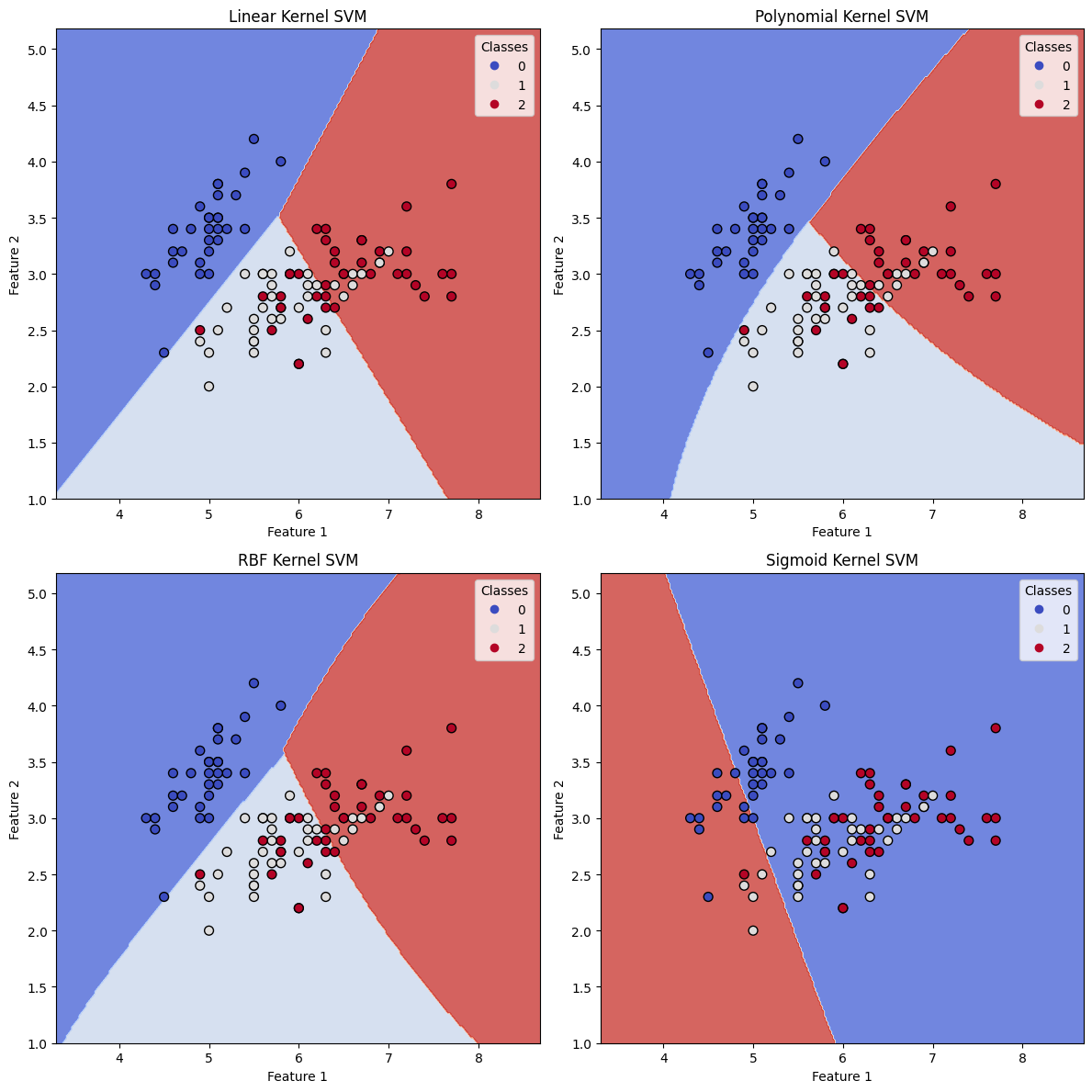
By running the above code, we obtain four plots showing the decision boundaries of the SVM models with different kernels. The plots illustrate how each kernel leads to different decision boundaries, which in turn affect the classification results.

• The Linear kernel results in a linear decision boundary, which might not be suitable for complex datasets with nonlinear patterns.
• The Polynomial kernel allows for more flexibility by creating curved decision boundaries, which can better fit the data when linear separation is not possible. The degree of the polynomial can be adjusted to control the complexity of the decision boundary.
• The RBF (Radial Basis Function) kernel is a very popular choice for many classification problems, as it can handle complex, nonlinear patterns in the data. The decision boundaries are very smooth and adapt well to the underlying structure of the dataset.
• The Sigmoid kernel can also create non-linear decision boundaries, but it is generally less popular compared to the RBF kernel.

From the accuracy scores and the plots, we can observe how different kernel functions impact the performance of the SVM classifier. Depending on the nature of the dataset and the underlying patterns, an appropriate kernel should be chosen to achieve the best classification results.

References

https://www.analyticsvidhya.com/blog/2017/09/understaing-support-vector-machine-example-code/?utm_source=blog&utm_medium=support-vector-regression-tutorial-for-machine-learning
https://towardsdatascience.com/support-vector-machine-introduction-to-machine-learning-algorithms-934a444fca47
https://medium.com/@zxr.nju/what-is-the-kernel-trick-why-is-it-important-98a98db0961d