What is a loss function?

In machine learning, the loss function is a function to calculate the size of the discrepancy between the "predicted value" output by the model and the actual "correct value. In other words, the loss function is an indicator of the "badness" of the model, that is, how poorly the model fits the data. In training a neural network, the model is optimized by searching for parameters (weights and biases) that minimize the loss function.

There are a variety of loss functions. The following are examples

• Mean Squared Error (MSE)
• Mean Absolute Error (MAE)
• Root Mean Square Error (RMSE)
• Logarithmic Mean Square Error (MSLE)
• Cross-entropy error
• Huber Loss
• Poisson Loss

In this article, I will introduce the Mean Square Error and Cross Entropy Error.

Mean Squared Error

The mean squared error is the difference between the output value and the correct value squared and summed over all output layer neurons. The mean squared error is defined by the following equation where E is the error, y_k is each output value in the output layer and t_k is the correct answer value.

Mean squared error is often used in regression problems because it is suited to cases where the correct answer or output is a continuous number.

Using Python, the mean squared error can be implemented as follows.

def square_sum(y, t):
    return 1.0/2.0 * np.sum(np.square(y - t))

Let's test this function with an example of handwriting digit recognition. First, prepare the following output values for the softmax function.

y = np.array([0.1, 0,6, 0,2, 0.05, 0.05, 0, 0, 0, 0, 0])

The output of the softmax function can be interpreted as a probability, which means that the probability of "0" is 0.1 and the probability of "1" is 0.6.

Next, we prepare the correct answer data. Here, we prepare the correct answer data for the cases where the correct answer for handwriting digit recognition is "0" and "1", respectively.

t1 = np.array([1, 0, 0, 0, 0, 0, 0, 0, 0, 0])
t2 = np.array([0, 1, 0, 0, 0, 0, 0, 0, 0, 0])

The correct data is a one-hot representation, where the correct label is represented by 1 and all other labels are represented by 0.

The mean squared error is calculated using the output values and the correct answer data.

import numpy as np

def square_sum(y, t):
    return 1.0/2.0 * np.sum(np.square(y - t))

y = np.array([0.1, 0.6, 0.2, 0.05, 0.05, 0, 0, 0, 0, 0])

t1 = np.array([1, 0, 0, 0, 0, 0, 0, 0, 0, 0])
t2 = np.array([0, 1, 0, 0, 0, 0, 0, 0, 0, 0])

print('y and t1:', square_sum(y, t1))
print('y and t2:', square_sum(y, t2))

y and t1: 0.6074999999999999
y and t2: 0.10750000000000003

Since output y has the highest probability of being "1", we see that the error with t2, where "1" is the correct label, is smaller.

Cross-Entropy Error

Cross-entropy error is a measure of the discrepancy between two distributions and is often used in classification problems. The cross-entropy error is expressed by the following equation.

The correct answer value in the classification problem is a one-hot representation, where the correct answer level is represented by 1 and all other values are represented by 0. Therefore, only terms with t_k of 1 in \sum on the right-hand side will affect the error, and the effect of terms with t_k of 0 will be ignored.

Let's think about \log (y_k). The natural logarithm \log x has the property that it becomes "0" when x is 1 and becomes infinitely small as x approaches 0. Taking the absolute value of the natural logarithm, the graph of -\log x against the output y of the neural network is as follows.

%matplotlib inline

import matplotlib.pyplot as plt
y = np.arange(0, 1.01, 0.01)
delta = 1e-7
loss = -np.log(y + delta)
plt.plot(y, loss)
plt.xlim(0, 1)
plt.xlabel('x')
plt.ylim(0, 5)
plt.ylabel('- log x')
plt.show()

-\log x is 0 when x is 1 and grows infinitely large as x approaches 0. In other words, the closer the output is to the correct answer, the closer the error is to 0, and the further the output is away from the correct answer, the farther the error is from 0. Thus, the cross-entropy error uses the natural logarithm property to derive the loss function.

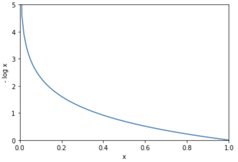
Cross-entropy has the advantage of fast learning speed when the isolation between the output and correct values is large. As noted above, learning is fast in such cases because t the error grows infinitely when the output is isolated from the correct answer.

Cross-entropy error can be implemented in Python as follows.

import numpy as np

def cross_entropy(y, t):
    return - np.sum(t * np.log(y + 1e-7))

The reason for adding the minute value 1e-7 to y is to prevent the contents of the log function from being zero and the natural logarithm from diverging to infinity.

Calculate the cross-entropy error using the output and correct data used in the mean squared error example.

import numpy as np

def cross_entropy(y, t):
    return - np.sum(t * np.log(y + 1e-7))

y = np.array([0.1, 0.6, 0.2, 0.05, 0.05, 0, 0, 0, 0, 0])

t1 = np.array([1, 0, 0, 0, 0, 0, 0, 0, 0, 0])
t2 = np.array([0, 1, 0, 0, 0, 0, 0, 0, 0, 0])

print('y and t1:', cross_entropy(y, t1))
print('y and t2:', cross_entropy(y, t2))

y and t1: 2.302584092994546
y and t2: 0.510825457099338

We could express the error between the output and the correct data as a loss function!