


What is Gradient Boosting Decision Trees (GBDT)
Gradient Boosting Decision Trees (GBDT) is a powerful ensemble learning method that combines the strengths of decision trees and gradient boosting techniques. It has become increasingly popular in recent years due to its ability to deliver high-performance models that can handle a wide range of complex problems in various domains, including finance, healthcare, and marketing.
GBDT works by iteratively constructing a series of decision trees, where each tree attempts to correct the errors made by its predecessor. This process continues until a specified number of trees have been created or a predefined level of performance has been reached. By combining the predictions of multiple trees, GBDT can often achieve better accuracy and generalization than a single decision tree.
GBDT Algorithm
In this section, I will explore the GBDT algorithm, focusing on both regression and classification cases. The main idea behind GBDT is to build a sequence of weak decision trees, where each tree is trained to correct the errors made by its predecessor. By iteratively improving the model, GBDT can achieve high accuracy and generalization. Let's delve into the main components of the GBDT algorithm.
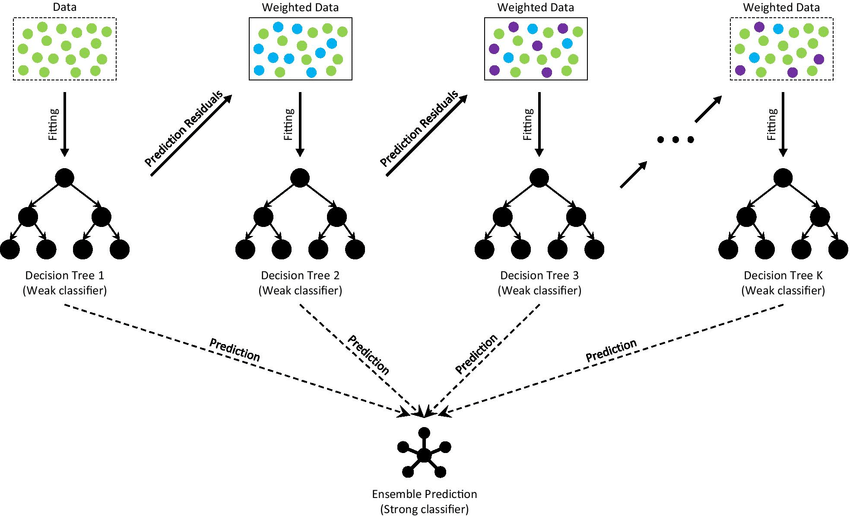
The architecture of Gradient Boosting Decision Tree
- Initialize the model with a constant prediction
GBDT starts by initializing the model with a constant prediction value. For regression problems, this constant is typically the mean of the target values, while for classification problems, it can be the log-odds of the majority class.
For regression, the initial prediction
For binary classification, the initial prediction
where
- Iteratively build decision trees
GBDT builds a sequence of decision trees by iteratively fitting a new tree to the pseudo-residuals (gradients) of the loss function. The pseudo-residuals are calculated as the negative gradient of the loss function with respect to the current model's predictions. This guides the algorithm towards a better approximation of the target function by minimizing the loss.
For regression with a least-squares loss function, the pseudo-residuals
For binary classification with a logistic loss function, the pseudo-residuals
- Update the model with a weighted tree prediction
After building a new decision tree
- Stop the process
The algorithm continues to build and add decision trees until a predefined number of trees is reached or the improvement in performance becomes negligible.
GBDT vs. Random Forests
Both GBDT and Random Forests are ensemble methods that utilize decision trees as base learners, but there are some key differences between them:
-
Boosting vs. Bagging
GBDT is a boosting algorithm, where each tree is built sequentially to correct the errors of its predecessor. In contrast, Random Forests is a bagging algorithm, where trees are built independently using bootstrapped samples of the dataset. -
Tree structure
GBDT typically uses shallow trees, which are weak learners, while Random Forests employs deep, fully grown trees. -
Model complexity
GBDT models can be more complex than Random Forests due to the iterative nature of boosting. This can lead to better performance but also increases the risk of overfitting. -
Training speed
Training a GBDT model can be slower than training a Random Forest, as the trees must be built sequentially. However, GBDT models can often achieve similar or better performance with fewer trees, which can offset the increased training time. -
Interpretability
Both GBDT and Random Forest models are less interpretable than single decision trees, but GBDT models can be even more difficult to interpret due to the sequential construction of trees and the use of gradient information. -
Robustness to noisy data
Random Forests are generally more robust to noisy data, as they build multiple independent trees and average their predictions. GBDT, on the other hand, may be more sensitive to noise, as each tree is influenced by the errors of its predecessor. -
Hyperparameter tuning
GBDT typically requires more hyperparameter tuning than Random Forests to achieve optimal performance, as it involves additional parameters such as learning rate and regularization.
GBDT in Python
Here are the Python scripts for implementing GBDT models. California Housing dataset for regression and the Iris dataset for classification are used as examples.
Regression: California Housing dataset
import numpy as np
import pandas as pd
from sklearn.datasets import fetch_california_housing
from sklearn.model_selection import train_test_split
from sklearn.ensemble import GradientBoostingRegressor
from sklearn.metrics import mean_squared_error

data = fetch_california_housing()
X, y = data.data, data.target

# Split the dataset into training and testing sets
X_train, X_test, y_train, y_test = train_test_split(X, y, test_size=0.2, random_state=42)

# Create and train the GBDT model
gbdt_regressor = GradientBoostingRegressor(
    n_estimators=100,
    max_depth=3,
    learning_rate=0.1,
    random_state=42
)
gbdt_regressor.fit(X_train, y_train)

# Evaluate the model
y_pred = gbdt_regressor.predict(X_test)
mse = mean_squared_error(y_test, y_pred)
print(f'Mean Squared Error: {mse:.4f}')
Mean Squared Error: 0.2940
Classification: Iris dataset
from sklearn.datasets import load_iris

data = load_iris()
X, y = data.data, data.target

# Split the dataset into training and testing sets
X_train, X_test, y_train, y_test = train_test_split(X, y, test_size=0.2, random_state=42)

from sklearn.ensemble import GradientBoostingClassifier
from sklearn.metrics import accuracy_score

# Create and train the GBDT model
gbdt_classifier = GradientBoostingClassifier(
    n_estimators=100,
    max_depth=3,
    learning_rate=0.1,
    random_state=42
)
gbdt_classifier.fit(X_train, y_train)

# Evaluate the model
y_pred = gbdt_classifier.predict(X_test)
accuracy = accuracy_score(y_test, y_pred)
print(f'Accuracy: {accuracy:.4f}')
Accuracy: 1.0000
References


Ryusei Kakujo


Weave the future of cities through data
Transportation modeling/ Urban planning/ Machine learning/ Computer science/ GIS