


Introduction
In this article, I will demonstrate how to implement a random forest classifier using the Titanic dataset from the seaborn library.
Preparing the dataset
First, let's import the necessary libraries and load the Titanic dataset.
import numpy as np
import pandas as pd
import seaborn as sns
from sklearn.model_selection import train_test_split
from sklearn.preprocessing import LabelEncoder
from sklearn.ensemble import RandomForestClassifier
from sklearn.metrics import accuracy_score, classification_report, confusion_matrix
import matplotlib.pyplot as plt

# Load the dataset
data = sns.load_dataset('titanic')

# Drop unnecessary columns
data = data.drop(['deck', 'embark_town', 'alive', 'who', 'adult_male', 'class'], axis=1)

# Handle missing values
data['age'] = data['age'].fillna(data['age'].median())
data['embarked'] = data['embarked'].fillna(data['embarked'].mode()[0])

# Encode categorical variables
encoder = LabelEncoder()
data['sex'] = encoder.fit_transform(data['sex'])
data['embarked'] = encoder.fit_transform(data['embarked'])

# Split the dataset into training and testing sets
X = data.drop('survived', axis=1)
y = data['survived']
X_train, X_test, y_train, y_test = train_test_split(X, y, test_size=0.3, random_state=42)
Building the model
Next, we will create a random forest classifier using scikit-learn.
# Create a random forest classifier with additional hyperparameters
rf_clf = RandomForestClassifier(
    n_estimators=100,      # Number of trees in the forest
    criterion='gini',      # Function to measure the quality of a split ('gini' or 'entropy')
    max_depth=None,        # Maximum depth of the tree (None means nodes are expanded until all leaves are pure)
    min_samples_split=2,   # Minimum number of samples required to split an internal node
    min_samples_leaf=1,    # Minimum number of samples required to be at a leaf node
    max_features='auto',   # Number of features to consider when looking for the best split ('auto', 'sqrt', 'log2', or an integer)
    bootstrap=True,        # Whether bootstrap samples are used when building trees
    oob_score=False,       # Whether to use out-of-bag samples to estimate the generalization accuracy
    n_jobs=None,           # Number of jobs to run in parallel for both fit and predict (-1 means using all processors)
    random_state=42,       # Controls both the randomness of the bootstrapping and feature sampling
    verbose=0,             # Controls the verbosity when fitting and predicting
    warm_start=False,      # Reuse the solution of the previous call to fit and add more estimators to the ensemble
    class_weight=None      # Weights associated with classes (None or 'balanced')
)
Here is a brief explanation of the additional hyperparameters:
-
n_estimator
It represents the number of decision trees in the random forest ensemble. In other words, it controls the size of the forest by specifying how many individual trees should be built and combined. By default, the value is set to 100, which means the random forest will consist of 100 decision trees. -
criterion
The function used to measure the quality of a split. Supported criteria are"gini"for Gini impurity and"entropy"for information gain. By default, it's set to"gini". -
max_depth
The maximum depth of the tree. IfNone, then nodes are expanded until all leaves are pure or until all leaves contain less than min_samples_split samples. A higher value may lead to overfitting, while a lower value may result in underfitting. -
min_samples_split
The minimum number of samples required to split an internal node. Increasing this value may reduce overfitting but could result in a less accurate model. -
min_samples_leaf
The minimum number of samples required to be at a leaf node. Increasing this value may reduce overfitting but could result in a less accurate model. -
max_features
The number of features to consider when looking for the best split. It can be set to'auto','sqrt','log2', or an integer. If 'auto', thenmax_features=sqrt(n_features)is used. If'sqrt', thenmax_features=sqrt(n_features)is used. If'log2', thenmax_features=log2(n_features)is used. If an integer, then the number of features is considered at each split. -
bootstrap
Whether bootstrap samples are used when building trees. IfFalse, the whole dataset is used to build each tree. -
oob_score
Whether to use out-of-bag samples to estimate the generalization accuracy. Out-of-bag samples are those not used in the bootstrap sample for a particular tree. -
n_jobs
The number of jobs to run in parallel for both fit and predict.-1means using all processors. -
verbose
Controls the verbosity when fitting and predicting. A higher value will output more information during the process. -
warm_start
When set to True, reuse the solution of the previous call to fit and add more estimators to the ensemble. This can save time when tuning hyperparameters iteratively, as it reuses the previously trained trees and adds new ones, rather than training all trees from scratch. -
class_weight
Weights associated with classes. IfNone, all classes are supposed to have equal weight. If'balanced', the class weights are adjusted based on the number of samples in each class. This can be useful when dealing with imbalanced datasets.
Training and evaluation
Now, let's train the random forest classifier on the training data and evaluate its performance on the testing data.
# Train the model
rf_clf.fit(X_train, y_train)

# Make predictions on the test set
y_pred = rf_clf.predict(X_test)

# Evaluate the model
accuracy = accuracy_score(y_test, y_pred)
print(f"Accuracy: {accuracy:.2f}")
print("Classification Report:")
print(classification_report(y_test, y_pred))
print("Confusion Matrix:")
print(confusion_matrix(y_test, y_pred))
Accuracy: 0.78
Classification Report:
              precision    recall  f1-score   support

           0       0.80      0.83      0.81       157
           1       0.74      0.70      0.72       111

    accuracy                           0.78       268
   macro avg       0.77      0.77      0.77       268
weighted avg       0.77      0.78      0.78       268

Confusion Matrix:
[[130  27]
 [ 33  78]]
Visualizing feature importance
Finally, we will visualize the feature importance of the random forest model.
# Calculate feature importances
importances = rf_clf.feature_importances_

# Sort feature importances in descending order
indices = np.argsort(importances)[::-1]

# Rearrange feature names so they match the sorted feature importances
names = [X.columns[i] for i in indices]

# Create a bar plot
plt.figure(figsize=(10, 5))
plt.title("Feature Importance")
plt.bar(range(X.shape[1]), importances[indices])

# Add feature names as x-axis labels
plt.xticks(range(X.shape[1]), names, rotation=90)

# Show the plot
plt.show()
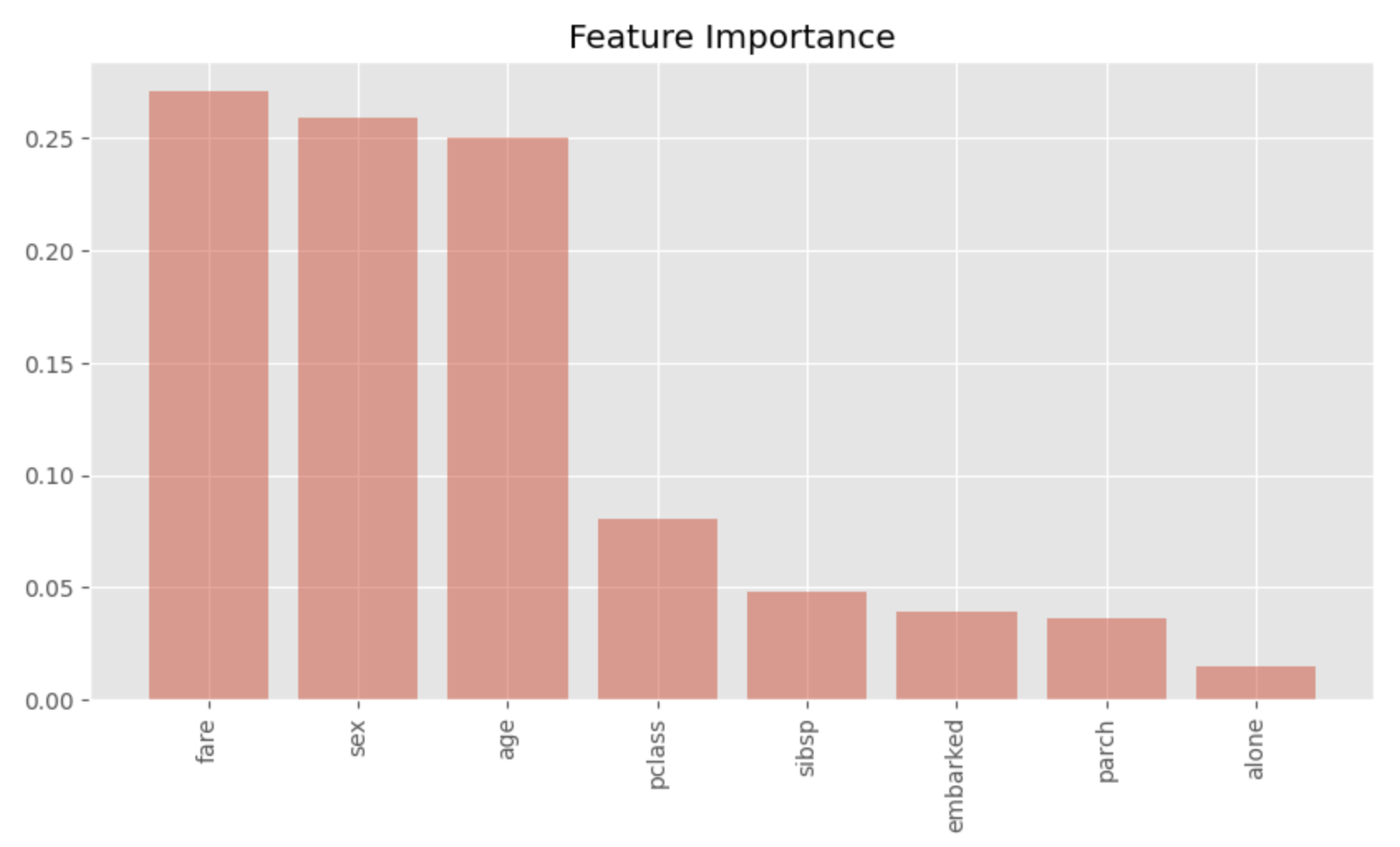
Plotting in this way, we can see at a glance which features are important. We can see that sex, age and fare are highly important. This is a convincing result as an important factor that made the difference between life and death on the Titanic.


Ryusei Kakujo


Weave the future of cities through data
Transportation modeling/ Urban planning/ Machine learning/ Computer science/ GIS