2022-11-04

Optimization algorithm

What is an optimization algorithm?

The goal of training a neural network is to find a parameter that minimizes the value of the loss function as much as possible. An optimization algorithm is an algorithm to efficiently arrive at this minimum value of loss.

Optimization algorithms are often compared to adventurers. The idea is to reach the bottom of the deepest valley in a vast area of land while blindfolded, without looking at a map. Because we are blindfolded, we rely only on the slope under our feet to reach the bottom of the valley. The player must sense the slope of the land and devise a strategy to reach the bottom of the valley. If the strategy is not correct, you may end up at a localized depression or take a detour to reach the bottom of the valley. How to reach the correct minimum efficiently is important.

Gradient descent method

The gradient descent method is a method of differentiating a loss function by a parameter, searching for a direction to reduce the loss, and adjusting the parameter in that direction. The gradient descent method repeats the following steps.

input data to the neural network and output predictions
define a loss function for the correct and predicted values
differentiate the loss function with a parameter
update the parameters with the differentiated values

This step can be expressed in a mathematical formula as follows.

w_{t+1} = w_t-\eta\frac{\partial L}{\partial w_t}

Here $w$ denotes the parameter for the $t$ th update, $L$ denotes the loss function, $\frac{\partial L}{\partial w}$ is the gradient of the loss function with respect to $w$ , and $\eta$ is a hyperparameter called the learning rate. The equation for updating the parameters is called the update equation.

Parameter updating requires the following two decisions

Whether to increase or decrease the value of the parameter
How much to change the value of the parameter

The first is determined by the derivative of the gradient. The second is determined by the learning rate.

The gradient descent method can be divided into the following three types depending on the amount of data used

Batch gradient descent
SGD (stochastic gradient descent)
Mini-batch SGD

Batch gradient descent

The batch gradient descent method searches for the minimum value of the loss function using all data. This means that the batch gradient descent method is used for the average of all data.

While the batch gradient descent method can update parameters all at once, it has the following disadvantages

It is computationally expensive.
It is difficult to get out when stuck in a locally optimal solution

Among the disadvantages, the large amount of computation can be solved by parallel computation. However, it is inevitable that when stuck in a locally optimal solution, there is no way out. A locally optimal solution is a minimum value that is not a minimum. If the same data is used for each parameter update, it is impossible to get out of a local optimum once it falls into a local minimum because the exact same data is put into the local optimum. SGD solves this problem.

SGD (Stochastic gradient descent)

SGD (Stochastic gradient descent) is an algorithm that randomly selects data for each parameter update. While the batch gradient descent method uses all data for a single parameter update, SGD uses only one randomly picked piece of data for each update. Therefore, SGD eliminates the problem of convergence to a locally optimal solution that can occur in the batch gradient descent method by randomly selecting a sample for each $w$ update. It also has the advantage of efficiently learning from redundancies in the training data.

One disadvantage of SGD is that it cannot be parallelized and learning is slow because it cannot move to the next data unless it is updated with gradients from one set of data.

Mini-batch SGD

Mini-batch SGD is a method between SGD and batch gradient descent. It uses a portion of the data to search for the minimum value of the loss function.

The batch gradient descent method calculates the gradient of all the data, so its calculation can be parallelized. On the other hand, SGD cannot parallelize the computation because the number of data for gradient computation is one. Therefore, mini-batch SGD, which uses a fixed number of data for training, can achieve parallelization while maintaining randomness. In other words, mini-batch SGD is a method that falls between the batch gradient descent method and SGD. The batch size of mini-batch SGD is a hyper-parameter, often 16 or 32.

However, even with mini-batch SGD, there is a problem that when searching for the minimum value of the loss function, it falls into a depression called pathological curvature, causing overshooting (oscillations that occur when a single update is too large) and slow learning. To illustrate this oscillation problem, consider the problem of finding the minimum of the following function.

f(x,y) = \frac{1}{20}x^2 + y^2

This function has the shape of an ellipse extending along the $x$ -axis. The gradient of the function is small along the $x$ -axis and large along the $y$ -axis. The minimum value of this function is $(x, y) = (0,0)$ . Start the search from $(x, y) = (-7,2)$ and apply SGD. The code is as follows.

import numpy as np
import matplotlib.pyplot as plt

class SGD:
    def __init__(self, lr=0.01):
        self.lr = lr

    def update(self, params, grads):
        for key in params.keys():
            params[key] -= self.lr * grads[key]


def f(x, y):
    return x**2 / 20.0 + y**2

def df(x, y):
    return x / 10.0, 2.0*y

init_pos = (-7.0, 2.0)
params = {}
params['x'], params['y'] = init_pos[0], init_pos[1]
grads = {}
grads['x'], grads['y'] = 0, 0

optimizer = SGD(lr=0.95)

x_history = []
y_history = []
params['x'], params['y'] = init_pos[0], init_pos[1]

for i in range(30):
    x_history.append(params['x'])
    y_history.append(params['y'])

    grads['x'], grads['y'] = df(params['x'], params['y'])
    optimizer.update(params, grads)

x = np.arange(-10, 10, 0.01)
y = np.arange(-5, 5, 0.01)

X, Y = np.meshgrid(x, y)
Z = f(X, Y)

# for simple contour line
mask = Z > 7
Z[mask] = 0

# plot
plt.figure(figsize=(12,6))
plt.plot(x_history, y_history, 'o-', color="red")
plt.contour(X, Y, Z)
plt.ylim(-10, 10)
plt.xlim(-10, 10)
plt.plot(0, 0, '+')
plt.title("SGD")
plt.xlabel("x")
plt.ylabel("y")

plt.show()

SGD

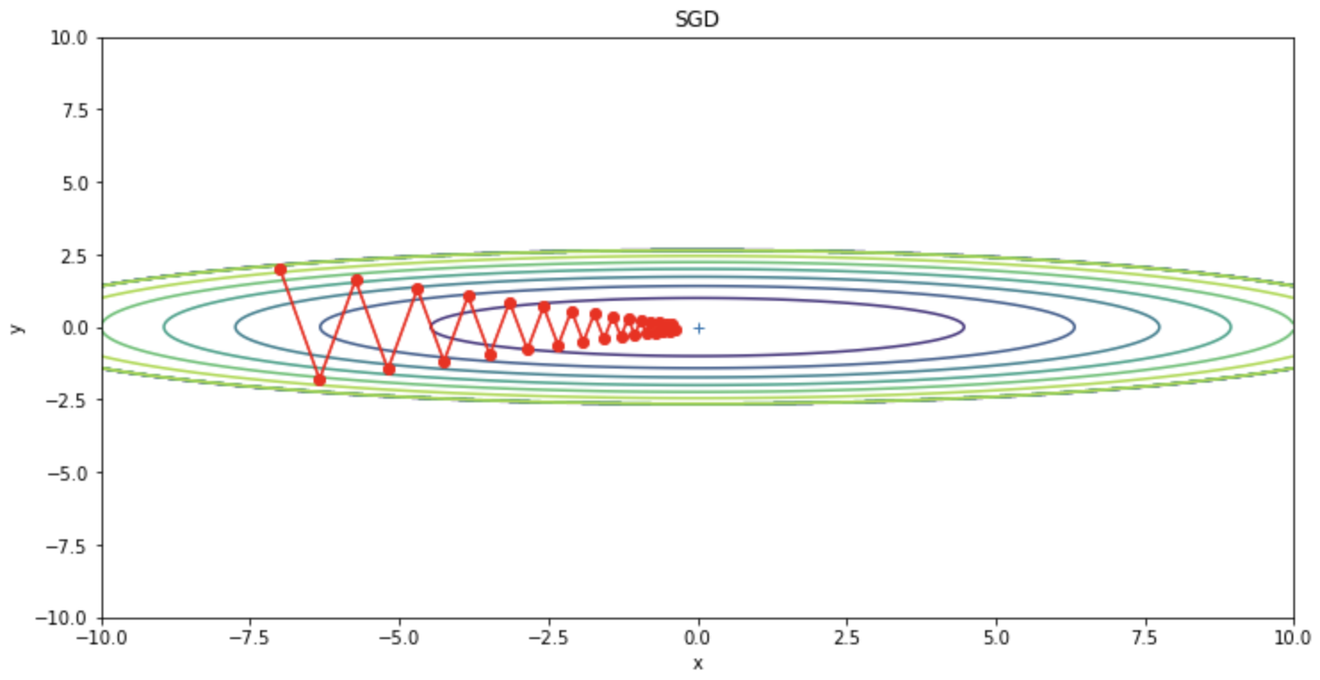
SGD can be seen to be oscillating in a zigzag manner. This oscillation is an inefficient path and is a factor that slows down learning. Thus, if the shape of the function is not isotropic, SGD will zigzag and search on inefficient paths.

To suppress this oscillation, Momentum, AdaGrad, and RMSProp, a modification of AdaGrad, are derived; Momentum from the derivative perspective, and AdaGrad and RMSProp from the learning rate perspective, using past gradient changes to suppress SDG oscillations.

Momentum

Momentum is an algorithm that adds a momentum (inertia term) to SGD. Momentum is a moving average of the gradient. Momentum is represented by the following update equation.

class Momentum:
    def __init__(self, lr=0.01, momentum=0.9):
        self.lr = lr
        self.momentum = momentum
        self.v = None

    def update(self, params, grads):
        if self.v is None:
            self.v = {}
            for key, val in params.items():
                self.v[key] = np.zeros_like(val)

        for key in params.keys():
            self.v[key] = self.momentum*self.v[key] - self.lr*grads[key]
            params[key] += self.v[key]

optimizer = Momentum(lr=0.1)

SMomentum

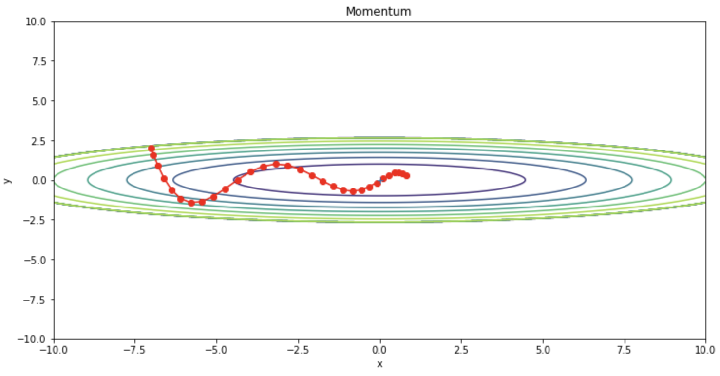
We can confirm that the oscillations are reduced compared to SGD.

AdaGrad

AdaGrad suppresses SGD oscillations by adjusting the learning rate. The following is the update formula for AdaGrad.

v_{t+1} = v_t + (\frac{\partial L}{\partial w_t})^2

w_{t+1} = w_t - \frac{\eta}{\sqrt{v_{t+1}}}\frac{\partial L}{\partial w_t}

The $v_{t+1}$ is the square of the gradient $\frac{\partial L}{\partial w_t}$ , which becomes larger when the change in gradient is large. Also, since $(\frac{\partial L}{\partial w_t})^2$ is always positive, $v_{t+1}$ increases with each update. Therefore, the learning rate $\frac{\eta}{\sqrt{v_{t+1}}}$ of the update amount $w_{t+1}$ becomes smaller when it is oscillating and also becomes smaller with each update. This makes it possible to search a large area at first and then gradually narrow down the search area for more efficient search.

The AdaGrad implementation code is shown below.

class AdaGrad:
    def __init__(self, lr=0.01):
        self.lr = lr
        self.h = None

    def update(self, params, grads):
        if self.h is None:
            self.h = {}
            for key, val in params.items():
                self.h[key] = np.zeros_like(val)

        for key in params.keys():
            self.h[key] += grads[key] * grads[key]
            params[key] -= self.lr * grads[key] / (np.sqrt(self.h[key]) + 1e-7)

optimizer = AdaGrad(lr=1.5)

AdaGrad

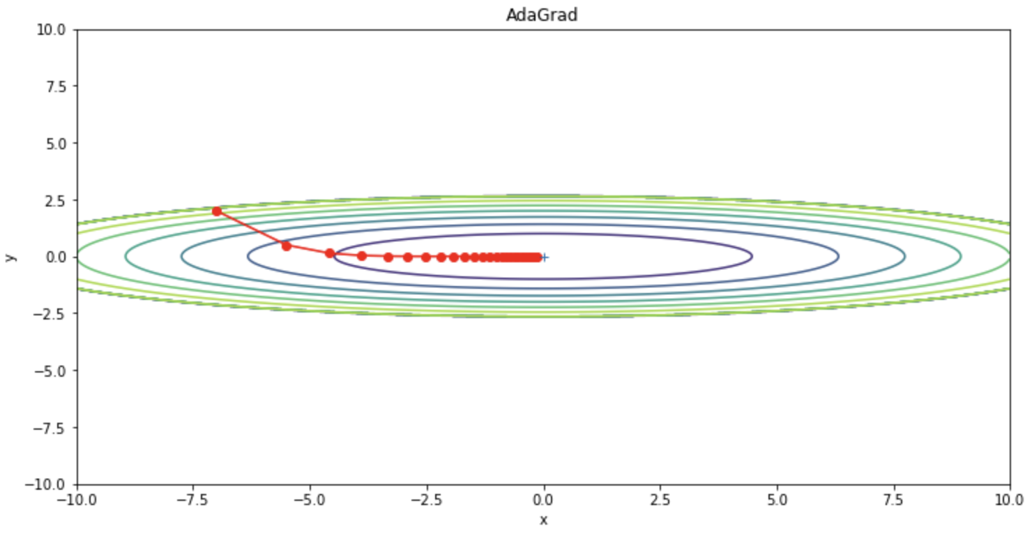
It can be seen that the oscillations are reduced compared to SGD.

On the other hand, AdaGrad has the disadvantage that the amount of updates is constantly decreasing, so the amount of updates may become almost zero in the middle of the process, causing the optimization to stop. In other words, if training is performed indefinitely, the amount of updates will reach zero and no updates will be performed at all. To remedy this problem, the RMSProp method was created.

RMSProp

RMSProp improves the problem of AdaGrad's slow learning due to low update rate.

v_{t+1} = \rho v_t + (1- \rho) (\frac{\partial L}{\partial w_t})^2

w_{t+1} = w_t - \frac{\eta}{\sqrt{v_{t+1}}}\frac{\partial L}{\partial w_t}

The $\rho$ reduces the learning rate so that more recent gradient information is reflected, rather than uniformly reflecting all past gradients.

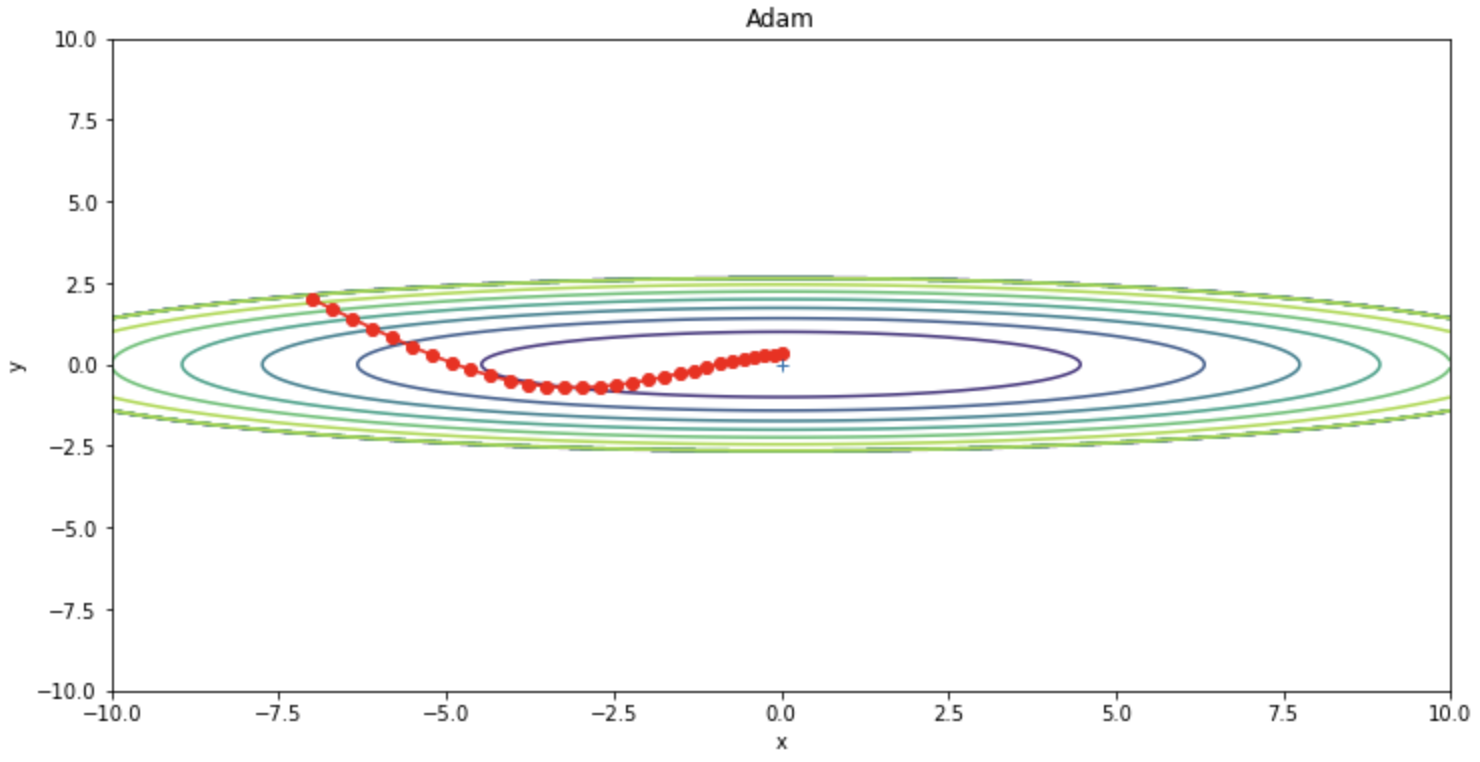
Adam

Adam (ADaptive Moment Estimation) is a fusion of Momentum and RMSProps and is a widely used optimization algorithm that often outperforms other optimization algorithms. The weights are updated as in the following update formula.

v_{t+1} = \beta v_t + (1- \beta)\frac{\partial L}{\partial w_t}

s_{t+1} = \rho v_t + (1- \rho) (\frac{\partial L}{\partial w_t})^2

w_{t+1} = w_t - \eta \frac{v_{t+1}}{\sqrt{s_{t+1}}}

The Adam implementation code is shown below.

class Adam:
    def __init__(self, lr=0.001, beta1=0.9, beta2=0.999):
        self.lr = lr
        self.beta1 = beta1
        self.beta2 = beta2
        self.iter = 0
        self.m = None
        self.v = None

    def update(self, params, grads):
        if self.m is None:
            self.m, self.v = {}, {}
            for key, val in params.items():
                self.m[key] = np.zeros_like(val)
                self.v[key] = np.zeros_like(val)

        self.iter += 1
        lr_t  = self.lr * np.sqrt(1.0 - self.beta2**self.iter) / (1.0 - self.beta1**self.iter)

        for key in params.keys():
            self.m[key] += (1 - self.beta1) * (grads[key] - self.m[key])
            self.v[key] += (1 - self.beta2) * (grads[key]**2 - self.v[key])
            params[key] -= lr_t * self.m[key] / (np.sqrt(self.v[key]) + 1e-7)

optimizer = Adam(lr=0.3)

Adam

Code summary

The following is a summary of the code used in this project.

import numpy as np
import matplotlib.pyplot as plt
from collections import OrderedDict

class SGD:
    """SGD"""
    def __init__(self, lr=0.01):
        self.lr = lr

    def update(self, params, grads):
        for key in params.keys():
            params[key] -= self.lr * grads[key]

class Momentum:
    """Momentum SGD"""
    def __init__(self, lr=0.01, momentum=0.9):
        self.lr = lr
        self.momentum = momentum
        self.v = None

    def update(self, params, grads):
        if self.v is None:
            self.v = {}
            for key, val in params.items():
                self.v[key] = np.zeros_like(val)

        for key in params.keys():
            self.v[key] = self.momentum*self.v[key] - self.lr*grads[key]
            params[key] += self.v[key]

class AdaGrad:
    """AdaGrad"""
    def __init__(self, lr=0.01):
        self.lr = lr
        self.h = None

    def update(self, params, grads):
        if self.h is None:
            self.h = {}
            for key, val in params.items():
                self.h[key] = np.zeros_like(val)

        for key in params.keys():
            self.h[key] += grads[key] * grads[key]
            params[key] -= self.lr * grads[key] / (np.sqrt(self.h[key]) + 1e-7)

class RMSprop:
    """RMSprop"""
    def __init__(self, lr=0.01, decay_rate = 0.99):
        self.lr = lr
        self.decay_rate = decay_rate
        self.h = None

    def update(self, params, grads):
        if self.h is None:
            self.h = {}
            for key, val in params.items():
                self.h[key] = np.zeros_like(val)

        for key in params.keys():
            self.h[key] *= self.decay_rate
            self.h[key] += (1 - self.decay_rate) * grads[key] * grads[key]
            params[key] -= self.lr * grads[key] / (np.sqrt(self.h[key]) + 1e-7)

class Adam:
    """Adam (http://arxiv.org/abs/1412.6980v8)"""
    def __init__(self, lr=0.001, beta1=0.9, beta2=0.999):
        self.lr = lr
        self.beta1 = beta1
        self.beta2 = beta2
        self.iter = 0
        self.m = None
        self.v = None

    def update(self, params, grads):
        if self.m is None:
            self.m, self.v = {}, {}
            for key, val in params.items():
                self.m[key] = np.zeros_like(val)
                self.v[key] = np.zeros_like(val)

        self.iter += 1
        lr_t  = self.lr * np.sqrt(1.0 - self.beta2**self.iter) / (1.0 - self.beta1**self.iter)

        for key in params.keys():
            self.m[key] += (1 - self.beta1) * (grads[key] - self.m[key])
            self.v[key] += (1 - self.beta2) * (grads[key]**2 - self.v[key])
            params[key] -= lr_t * self.m[key] / (np.sqrt(self.v[key]) + 1e-7)

def f(x, y):
    return x**2 / 20.0 + y**2

def df(x, y):
    return x / 10.0, 2.0*y

init_pos = (-7.0, 2.0)
params = {}
params['x'], params['y'] = init_pos[0], init_pos[1]
grads = {}
grads['x'], grads['y'] = 0, 0


optimizers = OrderedDict()
optimizers["SGD"] = SGD(lr=0.95)
optimizers["Momentum"] = Momentum(lr=0.1)
optimizers["AdaGrad"] = AdaGrad(lr=1.5)
# optimizers["RMSprop"] = RMSprop(lr=1.5)
optimizers["Adam"] = Adam(lr=0.3)

idx = 1

for key in optimizers:
    optimizer = optimizers[key]
    x_history = []
    y_history = []
    params['x'], params['y'] = init_pos[0], init_pos[1]

    for i in range(30):
        x_history.append(params['x'])
        y_history.append(params['y'])

        grads['x'], grads['y'] = df(params['x'], params['y'])
        optimizer.update(params, grads)


    x = np.arange(-10, 10, 0.01)
    y = np.arange(-5, 5, 0.01)

    X, Y = np.meshgrid(x, y)
    Z = f(X, Y)

    # for simple contour line
    mask = Z > 7
    Z[mask] = 0

    # plot
    plt.figure(figsize=(12,6))
    # plt.subplot(2, 2, idx)
    idx += 1
    plt.plot(x_history, y_history, 'o-', color="red")
    plt.contour(X, Y, Z)
    plt.ylim(-10, 10)
    plt.xlim(-10, 10)
    plt.plot(0, 0, '+')
    plt.title(key)
    plt.xlabel("x")
    plt.ylabel("y")

plt.show()