What is Vanishing Gradient Problem

The vanishing gradient problem is a well-known issue that occurs in deep neural networks during training. The problem arises when the gradients used to update the parameters of the network become very small as they propagate backward through the layers of the network. This can cause the early layers in the network to receive almost no update during training, leading to slow convergence and poor performance.

To understand the vanishing gradient problem, it is helpful to consider the backpropagation algorithm, which is used to train deep neural networks. During training, the backpropagation algorithm computes the gradient of the loss function with respect to the parameters of the network. This gradient is then used to update the parameters, allowing the network to learn from the training data.

However, in deep neural networks, the gradients can become very small as they propagate backward through the layers of the network. This occurs because the gradients are multiplied by the weight matrix at each layer, and the product of many small numbers can become extremely small. As a result, the early layers in the network receive almost no update during training, which leads to slow convergence and poor performance.

Causes of the Vanishing Gradient Problem

Choice of Activation Function

One significant factor that contributes to the vanishing gradient problem is the choice of activation function. Activation functions such as the sigmoid and hyperbolic tangent functions are prone to saturation, where the output becomes insensitive to small changes in the input. This saturation can cause the gradients to become very small, especially in deep networks with many layers. As a result, the early layers in the network receive almost no update during training, leading to slow convergence and poor performance.

To address this problem, researchers have proposed alternative activation functions that are less prone to saturation, such as the Rectified Linear Unit (ReLU) function. The ReLU function has a simple form and is easy to compute, making it popular in many deep learning applications. Additionally, recent research has explored more complex activation functions such as the Swish function, which has been shown to improve the performance of deep neural networks.

Network Depth

Another factor that can contribute to the vanishing gradient problem is the depth of the network. As the number of layers in the network increases, the gradients must propagate through more layers, which increases the likelihood of them becoming vanishingly small. This can make it challenging to train deep neural networks, as the gradients may become too small to be useful.

To address this problem, researchers have proposed techniques such as skip connections, where the output of one layer is added to the input of a later layer. Skip connections can help alleviate the vanishing gradient problem by allowing gradients to propagate more easily through the network. Additionally, normalization techniques such as batch normalization can help stabilize the gradients, allowing them to propagate more easily through the network.

Weight Initialization

Finally, the initialization of the weights in the network can also contribute to the vanishing gradient problem. If the weights are initialized to large values, the gradients can become very small as they propagate through the layers. This is because the product of large numbers can quickly become too large or too small, depending on the sign of the weights.

To address this problem, researchers have proposed careful weight initialization strategies such as Xavier initialization. Xavier initialization sets the initial weights of each layer to be proportional to the square root of the number of inputs to the layer. This ensures that the initial gradients are of appropriate magnitude, allowing them to propagate more easily through the network.

Effects of the Vanishing Gradient Problem

Slow Convergence During Training

One significant effect of the vanishing gradient problem is slow convergence during training. When the gradients become very small as they propagate backward through the network, the early layers in the network receive almost no update during training. This can lead to slow convergence and make it difficult to train the network effectively. In some cases, the network may not converge at all, preventing it from learning from the training data.

Potential for Suboptimal Solutions

Another effect of the vanishing gradient problem is the potential for the network to get stuck in a suboptimal solution. When the gradients become very small, the network may not be able to explore the entire space of possible solutions effectively. As a result, it may converge to a suboptimal solution that is not as good as the optimal solution. This can lead to poor performance on test data and limit the effectiveness of the network.

Overfitting Due to Vanishing Gradients

Finally, the vanishing gradient problem can also contribute to overfitting, where the network learns the training data too well and fails to generalize to new data. When the gradients become very small, the network may begin to overfit to the training data, memorizing the data rather than learning to generalize to new data. This can lead to poor performance on test data and limit the usefulness of the network in real-world applications.

Demonstrating the Vanishing Gradient Problem

In this chapter, I will demonstrate the vanishing gradient problem by showing the activation distribution.

We will use the PyTorch library to implement the deep neural network architecture and the MNIST dataset, which is a widely-used public dataset of handwritten digits. Our goal is to train a deep neural network to classify the digits correctly. We will use a deep neural network architecture with several hidden layers, each using the sigmoid activation function.

We will first train the network using the standard approach, without any techniques to address the vanishing gradient problem. We will then show the activation distributions at each layer of the network to demonstrate the impact of the vanishing gradient problem.

Here is the PyTorch code to define the deep neural network architecture and train the network:

import torch
import torch.nn as nn
import torch.optim as optim
import torchvision
import torchvision.transforms as transforms

# Load MNIST dataset
transform = transforms.Compose([transforms.ToTensor(), transforms.Normalize((0.5,), (0.5,))])
trainset = torchvision.datasets.MNIST(root='./data', train=True, download=True, transform=transform)
trainloader = torch.utils.data.DataLoader(trainset, batch_size=100, shuffle=True, num_workers=2)

# Define deep network with sigmoid activation
class DeepSigmoidNet(nn.Module):
    def __init__(self):
        super(DeepSigmoidNet, self).__init__()
        self.fc1 = nn.Linear(28 * 28, 1000)
        self.fc2 = nn.Linear(1000, 1000)
        self.fc3 = nn.Linear(1000, 1000)
        self.fc4 = nn.Linear(1000, 1000)
        self.fc5 = nn.Linear(1000, 1000)
        self.fc6 = nn.Linear(1000, 10)

    def forward(self, x):
        x = x.view(-1, 28 * 28)
        x = torch.sigmoid(self.fc1(x))
        x = torch.sigmoid(self.fc2(x))
        x = torch.sigmoid(self.fc3(x))
        x = torch.sigmoid(self.fc4(x))
        x = torch.sigmoid(self.fc5(x))
        x = self.fc6(x)
        return x

# Instantiate the network, loss function, and optimizer
net = DeepSigmoidNet()
criterion = nn.CrossEntropyLoss()
optimizer = optim.SGD(net.parameters(), lr=0.01, momentum=0.9)

# Train the network
for epoch in range(10):
    running_loss = 0.0
    for i, data in enumerate(trainloader, 0):
        inputs, labels = data
        optimizer.zero_grad()
        outputs = net(inputs)
        loss = criterion(outputs, labels)
        loss.backward()
        optimizer.step()
        running_loss += loss.item()

    # Print average loss per epoch
    print(f"Epoch {epoch + 1}, Loss: {running_loss / (i + 1)}")

# Collect gradients for histogram
gradients = []
for p in net.parameters():
    if p.grad is not None:
        gradients.append(p.grad.view(-1).cpu().numpy())

Let's draw the distribution of gradient values.

import numpy as np
import matplotlib.pyplot as plt

plt.style.use('ggplot')

# Create a histogram of the gradients
plt.hist(gradients, bins=100, range=(-1, 1), log=True, color='blue', alpha=0.5)
plt.xlabel('Gradient Values')
plt.ylabel('Frequency')
plt.title('Histogram of Gradient Values in Deep Sigmoid Network')
plt.show()

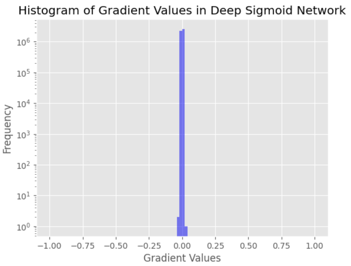
The vanishing gradient problem is found as a large number of very small gradient values, indicating that the gradients for the earlier layers in the network have almost vanished. This can lead to poor convergence and difficulties in training the network.