


What is RNN
RNN stands for Recurrent Neural Network. RNN is a type of neural network for processing sequences of input data, such as time series data or natural language, which is It is suitable for processing continuous input data, such as time-series data or natural language.
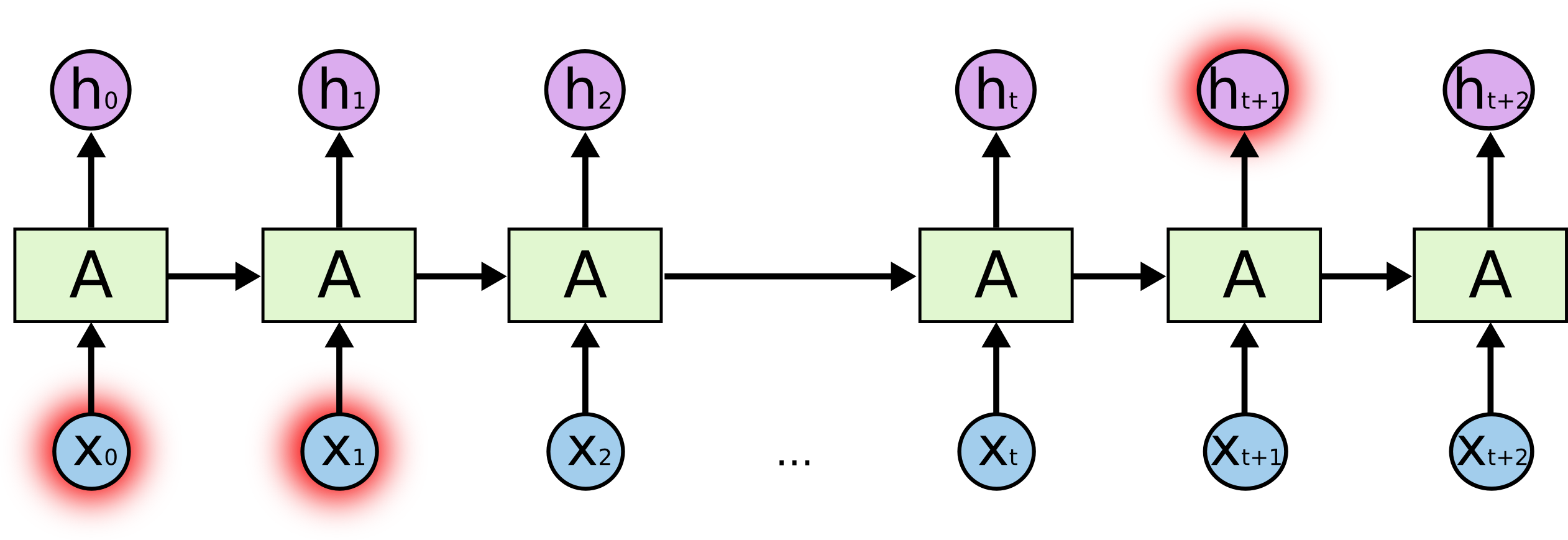
RNNs can take a sequence of input, such as time-series data, and process it with temporal dependencies in mind; RNNs, unlike traditional neural networks, can retain state for their input and convey the previous state to the next step. This allows the RNN to retain past information.
In the following RNN diagram, part of the output of the neural net at time
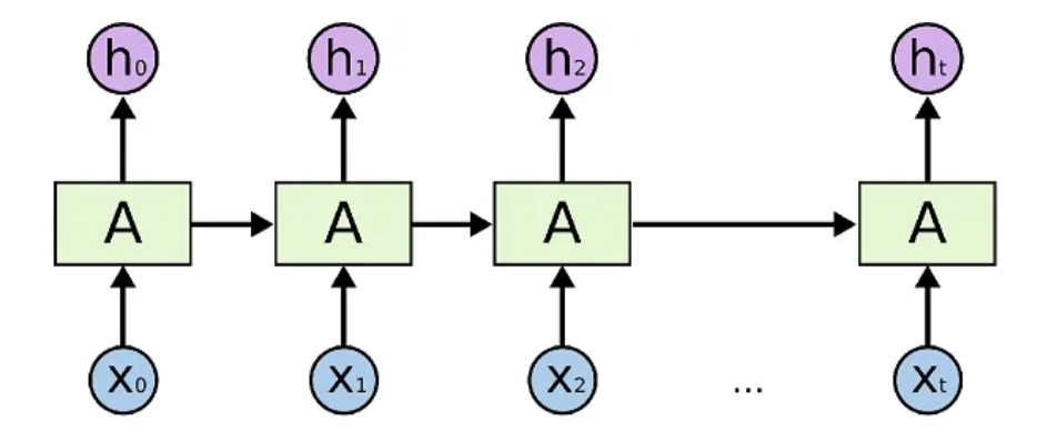
The main architectures of RNNs include simple RNNs, LSTMs, and GRUs. These architectures can store historical input data and combine it with the current input to produce output. These architectures are used for tasks such as time series data prediction, natural language processing, speech recognition, and image captioning.
A simple overview of RNN, LSTM and Attention Mechanism
Hidden state
The hidden state is a term used in fields such as machine learning and natural language processing to refer to unobserved states that a model maintains internally.
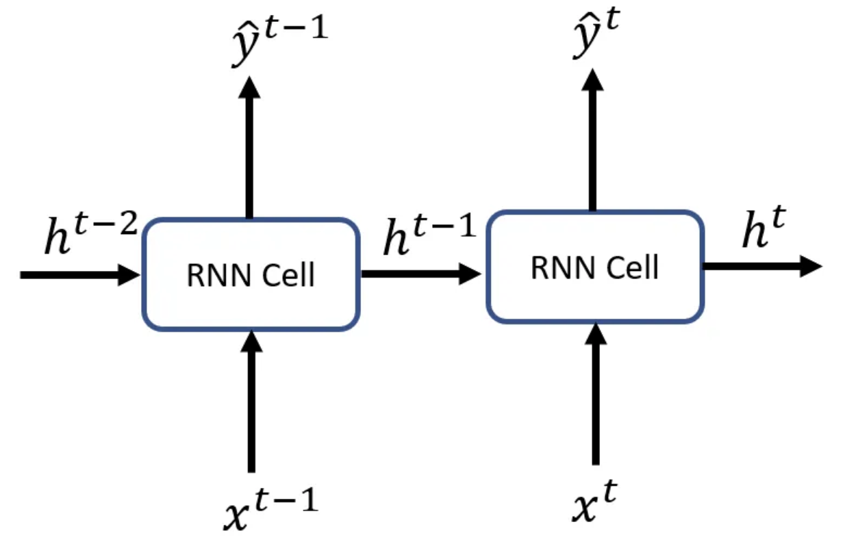
In RNNs, hidden states are computed from past inputs and their own outputs and are used to predict and process information about the next input. It converts the input sequence into a single vector and updates the hidden state based on it. The presence of hidden states makes the model more expressive for more complex problems and allows predictions that take into account the concept of time series.
The hidden state at
Since the output of a recurrent neuron at a given time step
Difference between hidden layer and hidden state
Hidden state and hidden layer are terms used in deep learning that are similar concepts, but have slightly different meanings.
Hidden state is a term used in models such as RNNs and LSTMs to describe the internal state, including the output at the previous time. in RNNs, hidden state is used to process time series data because it affects the input at the next time. In LSTMs, similarly, hidden state is used to preserve past information. The hidden layer is used to process time-series data, as it affects the input of the next time.
Hidden layers, on the other hand, are a term used in neural networks such as multilayer perceptrons (MLPs) to refer to the intermediate layer between the input and output layers. The hidden layer consists of multiple neurons, each of which receives signals from the previous layer, computes a weighted sum, and produces an output via an activation function. When there are multiple hidden layers, the output of each hidden layer is input to the next hidden layer or output layer.
In other words, hidden states and hidden layers are both concepts that represent internal states in machine learning, but they are used in different contexts and for different purposes. Hidden states are used to process time series data, while hidden layers represent the middle layer of a typical neural network.
RNN challenges
A major issue that makes RNN training very slow and inefficient is the gradient vanishing problem The process for a Feed Forward neural network is as follows
- output some result in the forward pass
- use that result to compute a loss value
- use that loss value to back propagate and compute gradients with respect to the weights
- back propagate these gradients with respect to the weights to fine tune the weights and improve the performance of the network
Because the weights are manipulated according to the previous layer, the small gradients tend to decrease significantly with each layer change and become very close to zero, resulting in poor learning in the early layers and overall ineffective learning.
A simple overview of RNN, LSTM and Attention Mechanism
Thus, if the gradient disappears, the RNN will not be able to learn long-range dependencies across time steps well. In other words, even if the initial input of a sequence is important to the overall context, it will not be important. Therefore, it cannot learn long sequences, resulting in short-term memory.
RNN Implementation
Here are some examples of RNN implementations using PyTorch and Keras.
PyTorch
The following is a basic example of using PyTorch to describe an RNN model. This example uses a simple RNN architecture to perform the task of classifying words.
import torch
import torch.nn as nn

class RNN(nn.Module):
    def __init__(self, input_size, hidden_size, output_size):
        super(RNN, self).__init__()

        self.hidden_size = hidden_size
        self.rnn = nn.RNN(input_size, hidden_size)
        self.fc = nn.Linear(hidden_size, output_size)

    def forward(self, input):
        hidden = torch.zeros(1, 1, self.hidden_size)
        output, hidden = self.rnn(input, hidden)
        output = self.fc(output[-1, :, :])
        return output
This model takes in words of size input_size, passes them through an RNN with a hidden layer size of hidden_size, and finally generates a classification output of size output_size. The nn.RNN class is the built-in RNN layer in PyTorch, and nn.Linear represents a fully connected layer.
The forward method performs the forward pass on the given input. First, the hidden layer is initialized. Then, the input and current hidden state are passed to the RNN to obtain the output and new hidden state. Finally, only the output from the last step is taken and passed through the fully connected layer to generate the classification output.
The link below is another example.
Keras
Let us implement RNN with Keras.
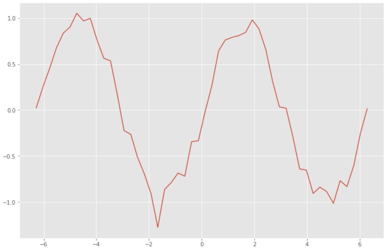
First, create training data for RNN. Create the data by adding noise to the sine function with random numbers.
%matplotlib inline

import numpy as np
import matplotlib.pyplot as plt


x_data = np.linspace(-2*np.pi, 2*np.pi)  # -2π to 2π
sin_data = np.sin(x_data)  + 0.1*np.random.randn(len(x_data))  # add noise to sin func

plt.style.use('ggplot')
plt.figure(figsize=(12, 8))
plt.plot(x_data, sin_data)
plt.show()

n_rnn = 10  # num of time series
n_sample = len(x_data)-n_rnn  # num of samples
x = np.zeros((n_sample, n_rnn))  # input
t = np.zeros((n_sample, n_rnn))  # label
for i in range(0, n_sample):
    x[i] = sin_data[i:i+n_rnn]
    t[i] = sin_data[i+1:i+n_rnn+1]

x = x.reshape(n_sample, n_rnn, 1)
t = t.reshape(n_sample, n_rnn, 1)
Build an RNN model to predict future values from past time-series data.
from keras.models import Sequential
from keras.layers import Dense, SimpleRNN

batch_size = 8  # batch size
n_in = 1  # num of neurons in input layer
n_mid = 20  # num of neurons in mid layer
n_out = 1  # num of neurons in output layer

model = Sequential()
model.add(SimpleRNN(n_mid, input_shape=(n_rnn, n_in), return_sequences=True))
model.add(Dense(n_out, activation="linear"))
model.compile(loss="mean_squared_error", optimizer="sgd")
print(model.summary())

>> Model: "sequential"
>> _________________________________________________________________
>>  Layer (type)                Output Shape              Param #
>> =================================================================
>>  simple_rnn (SimpleRNN)      (None, 10, 20)            440
>>
>>  dense (Dense)               (None, 10, 1)             21
>>
>> =================================================================
>> Total params: 461
>> Trainable params: 461
>> Non-trainable params: 0
>> _________________________________________________________________
>> None
Training is performed using the constructed RNN model.
history = model.fit(x, t, epochs=20, batch_size=batch_size, validation_split=0.1)

>> Epoch 1/20
>> 5/5 [==============================] - 2s 79ms/step - loss: 0.6561 - val_loss: 0.3590
>> Epoch 2/20
>> 5/5 [==============================] - 0s 13ms/step - loss: 0.4701 - val_loss: 0.2707
>> Epoch 3/20
>> 5/5 [==============================] - 0s 11ms/step - loss: 0.3694 - val_loss: 0.2240
>> Epoch 4/20
>> 5/5 [==============================] - 0s 11ms/step - loss: 0.3051 - val_loss: 0.1892
>> Epoch 5/20
>> 5/5 [==============================] - 0s 15ms/step - loss: 0.2613 - val_loss: 0.1696
>> Epoch 6/20
>> 5/5 [==============================] - 0s 13ms/step - loss: 0.2289 - val_loss: 0.1593
>> Epoch 7/20
>> 5/5 [==============================] - 0s 12ms/step - loss: 0.2058 - val_loss: 0.1501
>> Epoch 8/20
>> 5/5 [==============================] - 0s 12ms/step - loss: 0.1889 - val_loss: 0.1414
>> Epoch 9/20
>> 5/5 [==============================] - 0s 13ms/step - loss: 0.1750 - val_loss: 0.1345
>> Epoch 10/20
>> 5/5 [==============================] - 0s 14ms/step - loss: 0.1633 - val_loss: 0.1274
>> Epoch 11/20
>> 5/5 [==============================] - 0s 12ms/step - loss: 0.1540 - val_loss: 0.1233
>> Epoch 12/20
>> 5/5 [==============================] - 0s 12ms/step - loss: 0.1456 - val_loss: 0.1188
>> Epoch 13/20
>> 5/5 [==============================] - 0s 11ms/step - loss: 0.1377 - val_loss: 0.1133
>> Epoch 14/20
>> 5/5 [==============================] - 0s 12ms/step - loss: 0.1317 - val_loss: 0.1097
>> Epoch 15/20
>> 5/5 [==============================] - 0s 11ms/step - loss: 0.1256 - val_loss: 0.1063
>> Epoch 16/20
>> 5/5 [==============================] - 0s 11ms/step - loss: 0.1199 - val_loss: 0.1025
>> Epoch 17/20
>> 5/5 [==============================] - 0s 13ms/step - loss: 0.1152 - val_loss: 0.1025
>> Epoch 18/20
>> 5/5 [==============================] - 0s 11ms/step - loss: 0.1105 - val_loss: 0.0958
>> Epoch 19/20
>> 5/5 [==============================] - 0s 11ms/step - loss: 0.1065 - val_loss: 0.0932
>> Epoch 20/20
>> 5/5 [==============================] - 0s 15ms/step - loss: 0.1025 - val_loss: 0.0897
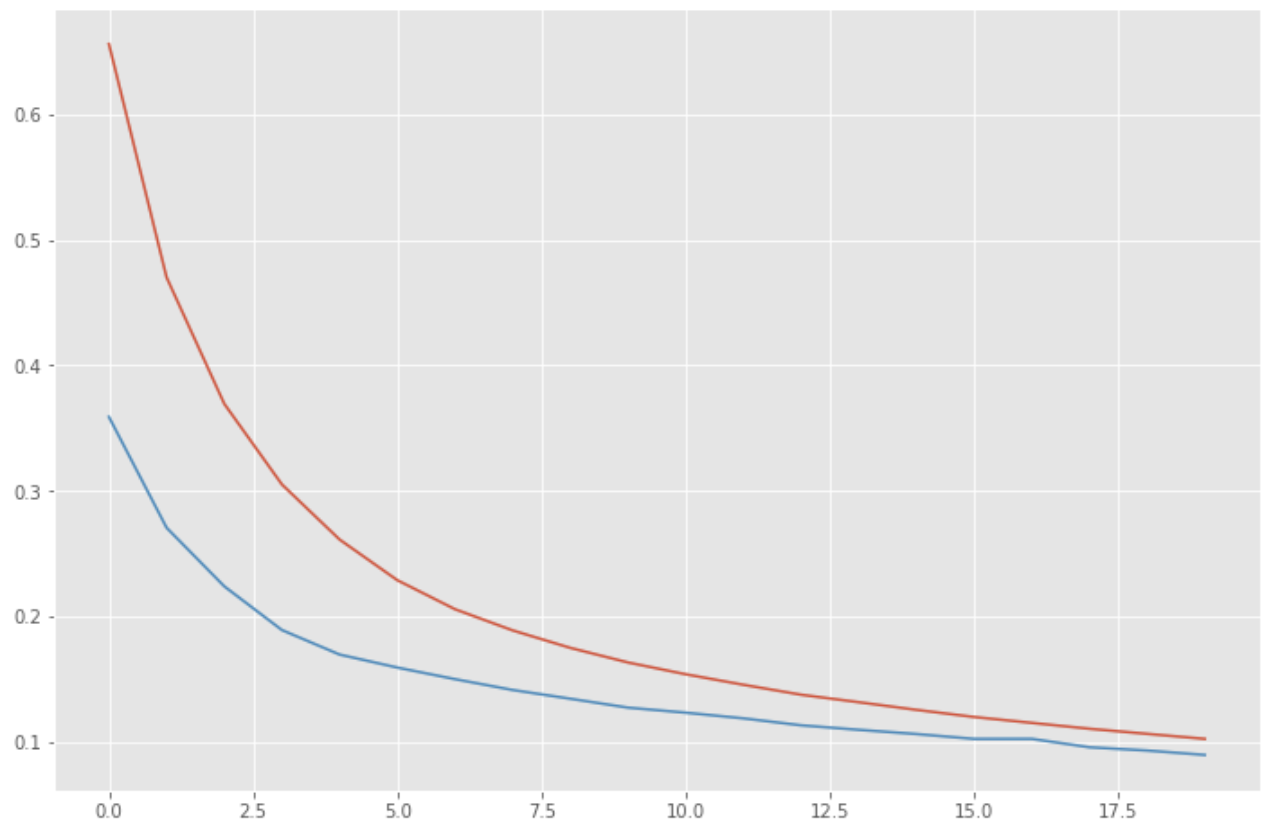
Check the error trend.
loss = history.history['loss']
vloss = history.history['val_loss']

plt.figure(figsize=(12, 8))
plt.plot(np.arange(len(loss)), loss)
plt.plot(np.arange(len(vloss)), vloss)
plt.show()
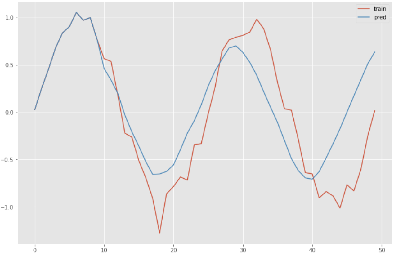
Predictions are made using the RNN's trained model.
predicted = x[0].reshape(-1)

for i in range(0, n_sample):
    y = model.predict(predicted[-n_rnn:].reshape(1, n_rnn, 1))
    predicted = np.append(predicted, y[0][n_rnn-1][0])

plt.figure(figsize=(12, 8))
plt.plot(np.arange(len(sin_data)), sin_data, label="training")
plt.plot(np.arange(len(predicted)), predicted, label="predicted")
plt.legend()
plt.show()
References


Ryusei Kakujo


Weave the future of cities through data
Transportation modeling/ Urban planning/ Machine learning/ Computer science/ GIS