

Introduction
The Tokyo Institute of Technology has created and maintains a collection of exercises on NLP called "NLP 100 Exercise".
In this article, I will find sample answers to "Chapter 7: Word Vector".
60. Loading word vectors
Download word vectors that are pretrained on Google News dataset (approx. 100 billion words). The file contains word vectors of 3 million words/phrases, whose dimentionalities are 300. Print out the word vector of the term “United States”. Note that “United States” is represented as “United_States” in the file.
from gensim.models import KeyedVectors

model = KeyedVectors.load_word2vec_format('./GoogleNews-vectors-negative300.bin.gz', binary=True)
print(model['United_States'])
[-3.61328125e-02 -4.83398438e-02  2.35351562e-01  1.74804688e-01
 -1.46484375e-01 -7.42187500e-02 -1.01562500e-01 -7.71484375e-02
 .
 .
 .
 -8.49609375e-02  1.57470703e-02  7.03125000e-02  1.62353516e-02
 -2.27050781e-02  3.51562500e-02  2.47070312e-01 -2.67333984e-02]
61. Word similarity
Compute the cosine similarity between “United States” and “U.S.”
model.similarity('United_States', 'U.S.')
0.73107743
62. Top-10 most similar words
Find the top-10 words that have the highest cosine similarity with the word “United States” and print out the similarity score.
model.most_similar('United_States', topn=10)
[('Unites_States', 0.7877248525619507),
 ('Untied_States', 0.7541370391845703),
 ('United_Sates', 0.74007248878479),
 ('U.S.', 0.7310774326324463),
 ('theUnited_States', 0.6404393911361694),
 ('America', 0.6178410053253174),
 ('UnitedStates', 0.6167312264442444),
 ('Europe', 0.6132988929748535),
 ('countries', 0.6044804453849792),
 ('Canada', 0.6019070148468018)]
63. Analogy based on the additive composition
Subtract the vector of “Madrid” from the vector of “Spain” and then add the vector of “Athens”. Compute the top-10 most similar words with the output vector.
model.most_similar(
  positive=['Spain', 'Athens'],
  negative=['Madrid'],
  topn=10
)
[('Greece', 0.6898480653762817),
 ('Aristeidis_Grigoriadis', 0.560684859752655),
 ('Ioannis_Drymonakos', 0.5552908778190613),
 ('Greeks', 0.545068621635437),
 ('Ioannis_Christou', 0.5400862097740173),
 ('Hrysopiyi_Devetzi', 0.5248445272445679),
 ('Heraklio', 0.5207759737968445),
 ('Athens_Greece', 0.516880989074707),
 ('Lithuania', 0.5166865587234497),
 ('Iraklion', 0.5146791338920593)]
64. Analogy data experiment
Download word analogy evaluation dataset. Compute the vector as follows: vec(word in second column) - vec(word in first column) + vec(word in third column). From the output vector, (1) find the most similar word and (2) compute the similarity score with the word. Append the most similar word and its similarity to each row of the downloaded file.
!wget http://download.tensorflow.org/data/questions-words.txt
!head -5 questions-words.txt

>> : capital-common-countries
>> Athens Greece Baghdad Iraq
>> Athens Greece Bangkok Thailand
>> Athens Greece Beijing China
>> Athens Greece Berlin Germany
with open('./questions-words.txt', 'r') as f1, open('./questions-words-add.txt', 'w') as f2:
  for line in f1:
    line = line.split()
    if line[0] == ':':
      category = line[1]
    else:
      word, cos = model.most_similar(positive=[line[1], line[2]], negative=[line[0]], topn=1)[0]
      f2.write(' '.join([category] + line + [word, str(cos) + '\n']))

!head -5 questions-words-add.txt

>> capital-common-countries Athens Greece Baghdad Iraq Iraqi 0.6351870894432068
>> capital-common-countries Athens Greece Bangkok Thailand Thailand 0.7137669324874878
>> capital-common-countries Athens Greece Beijing China China 0.7235777974128723
>> capital-common-countries Athens Greece Berlin Germany Germany 0.6734622120857239
>> capital-common-countries Athens Greece Bern Switzerland Switzerland 0.4919748306274414
65. Accuracy score on the analogy task
From the output of the problem 64, compute the accuracy score on both the semantic analogy and the syntactic analogy.
with open('./questions-words-add.txt', 'r') as f:
  sem_cnt = 0
  sem_cor = 0
  syn_cnt = 0
  syn_cor = 0
  for line in f:
    line = line.split()
    if not line[0].startswith('gram'):
      sem_cnt += 1
      if line[4] == line[5]:
        sem_cor += 1
    else:
      syn_cnt += 1
      if line[4] == line[5]:
        syn_cor += 1

print(f'semantic analogy accuracy: {sem_cor / sem_cnt:.3f}')
print(f'syntactic analogy accuracy: {syn_cor / syn_cnt:.3f}')

>> semantic analogy accuracy: 0.731
>> syntactic analogy accuracy: 0.740
66. Evaluation on WordSimilarity-353
Download the test data from The WordSimilarity-353 Test Collection. Compute the spearman’s rank correlation coefficient between two similarity rank scores: (1) similarity computed from word vectors and (2) similarity evaluated by the human.
!wget http://www.gabrilovich.com/resources/data/wordsim353/wordsim353.zip
!unzip wordsim353.zip
!head -5 './combined.csv'

>> Word 1,Word 2,Human (mean)
>> love,sex,6.77
>> tiger,cat,7.35
>> tiger,tiger,10.00
>> book,paper,7.46
import pandas as pd
import numpy as np
from scipy.stats import spearmanr

df = pd.read_csv('combined.csv')
df['sim'] = df.apply(lambda x: model.similarity(x['Word 1'], x['Word 2']), axis=1)
print(df.head(5))

correlation, pvalue = spearmanr(df['Human (mean)'], df['sim'])

print(f'\nspearman’s rank correlation : {correlation:.3f}')
print(f'pvalue : {pvalue}')

>>      Word 1    Word 2  Human (mean)       sim
>> 0      love       sex          6.77  0.263938
>> 1     tiger       cat          7.35  0.517296
>> 2     tiger     tiger         10.00  1.000000
>> 3      book     paper          7.46  0.363463
>> 4  computer  keyboard          7.62  0.396392
>>
>> spearman’s rank correlation : 0.700
>> pvalue : 2.86866666051422e-53
67. k-means clustering
Extract the word vectors of the country names. Apply k-means clustering where k=5.
from sklearn.cluster import KMeans

# get countries
countries = set()
with open('./questions-words-add.txt') as f:
  for line in f:
    line = line.split()
    if line[0] in ['capital-common-countries', 'capital-world']:
      countries.add(line[2])
    elif line[0] in ['currency', 'gram6-nationality-adjective']:
      countries.add(line[1])

# get country vectors
countries_vec = [model[country] for country in list(countries)]

# k-means clustering
kmeans = KMeans(n_clusters=5, random_state=42)
kmeans.fit(countries_vec)
for i in range(5):
  cluster = np.where(kmeans.labels_ == i)[0]
  print(f'cluster: {i}')
  print(', '.join([list(countries)[k] for k in cluster]))
cluster: 0
Rwanda, Uganda, Liberia, Burundi, Sudan, Somalia, Eritrea
cluster: 1
Australia, England, Sweden, Switzerland, Belgium, Denmark, Italy, Algeria, Portugal, France, Canada, Finland, Spain, Ireland, Norway, Germany
cluster: 2
Vietnam, Egypt, Lebanon, Iran, China, Qatar, Japan, Nepal, Pakistan, Iraq, Philippines, Thailand, Jordan, Indonesia, Bangladesh, Syria, Afghanistan, Bahrain
cluster: 3
Belarus, Slovenia, Ukraine, Kazakhstan, Serbia, Greece, Azerbaijan, Russia, Kyrgyzstan, Romania, Turkmenistan, Turkey, Moldova, Slovakia, Tajikistan, Hungary
cluster: 4
Jamaica, Guyana, Botswana, Malawi, Ghana, Nicaragua, Zambia, Venezuela, Mali, Samoa, Tuvalu, Madagascar, Belize, Guinea, Zimbabwe, Angola, Gabon, Gambia, Mozambique, Senegal, Nigeria, Peru, Cuba
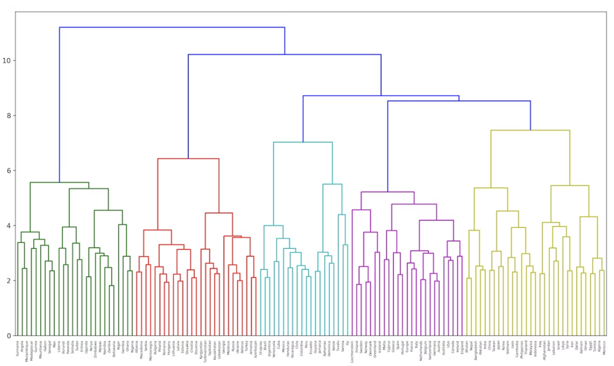
68. Ward’s method clustering
Apply hierarchical clustering to the word vectors of the country names. Use Ward’s method for the distance metric between two clusters. Visualize the clustering result as the dendrogram.
from matplotlib import pyplot as plt
from scipy.cluster.hierarchy import dendrogram, linkage

plt.figure(figsize=(15,5))
Z = linkage(countries_vec, method='ward')
dendrogram(Z, labels=countries)
plt.show()
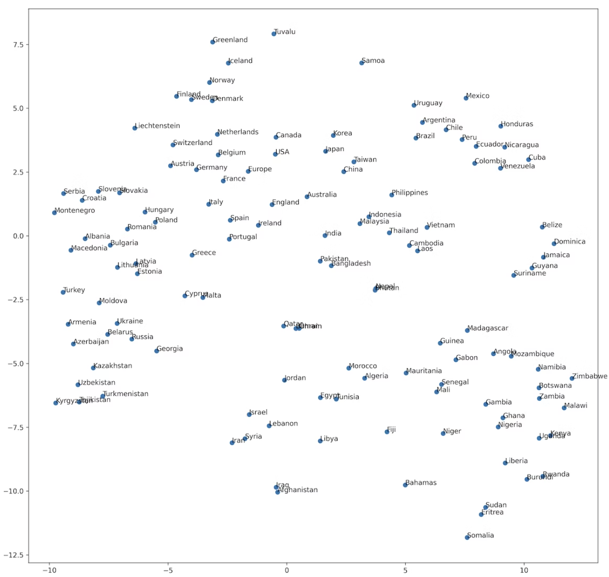
69. t-SNE Visualization
Visualize the word vector space of the country names by t-SNE.
!pip install bhtsne

import bhtsne

embedded = bhtsne.tsne(np.array(countries_vec).astype(np.float64), dimensions=2, rand_seed=123)
plt.figure(figsize=(10, 10))
plt.scatter(np.array(embedded).T[0], np.array(embedded).T[1])
for (x, y), name in zip(embedded, countries):
    plt.annotate(name, (x, y))
plt.show()
References


Ryusei Kakujo


Weave the future of cities through data
Transportation modeling/ Urban planning/ Machine learning/ Computer science/ GIS