2023-02-03

NLP 100 Exercise ch6：Machine Learning

Machine Learning

NLP

Introduction

The Tokyo Institute of Technology has created and maintains a collection of exercises on NLP called "NLP 100 Exercise".

https://nlp100.github.io/en/ch06.html

In this article, I will find sample answers to "Chapter 6: Machine Learning".

50. Download and Preprocess Dataset

Download News Aggregator Data Set and create training data (train.txt), validation data (valid.txt) and test data (test.txt) as follows:

Unpack the downloaded zip file and read readme.txt.

Extract the articles such that the publisher is one of the followings: “Reuters”, “Huffington Post”, “Businessweek”, “Contactmusic.com” and “Daily Mail”.

Randomly shuffle the extracted articles.

Split the extracted articles in the following ratio: the training data (80%), the validation data (10%) and the test data (10%). Then save them into files train.txt, valid.txt and test.txt, respectively. In each file, each line should contain a single instance. Each instance should contain both the name of the category and the article headline. Use Tab to separate each field.

After creating the dataset, check the number of instances contained in each category.

!wget https://archive.ics.uci.edu/ml/machine-learning-databases/00359/NewsAggregatorDataset.zip
!unzip ./NewsAggregatorDataset.zip

!wc -l ./newsCorpora.csv

>> 422937 ./newsCorpora.csv

!head -5 ./newsCorpora.csv

>> 1	Fed official says weak data caused by weather, should not slow taper	http://www.latimes.com/business/money/la-fi-mo-federal-reserve-plosser-stimulus-economy-20140310,0,1312750.story\?track=rss	Los Angeles Times	b	ddUyU0VZz0BRneMioxUPQVP6sIxvM	www.latimes.com	1394470370698
>> 2	Fed's Charles Plosser sees high bar for change in pace of tapering	http://www.livemint.com/Politics/H2EvwJSK2VE6OF7iK1g3PP/Feds-Charles-Plosser-sees-high-bar-for-change-in-pace-of-ta.html	Livemint	b	ddUyU0VZz0BRneMioxUPQVP6sIxvM	www.livemint.com	1394470371207
>> 3	US open: Stocks fall after Fed official hints at accelerated tapering	http://www.ifamagazine.com/news/us-open-stocks-fall-after-fed-official-hints-at-accelerated-tapering-294436	IFA Magazine	b	ddUyU0VZz0BRneMioxUPQVP6sIxvM	www.ifamagazine.com	1394470371550
>> 4	Fed risks falling 'behind the curve', Charles Plosser says	http://www.ifamagazine.com/news/fed-risks-falling-behind-the-curve-charles-plosser-says-294430	IFA Magazine	b	ddUyU0VZz0BRneMioxUPQVP6sIxvM	www.ifamagazine.com	1394470371793
>> 5	Fed's Plosser: Nasty Weather Has Curbed Job Growth	http://www.moneynews.com/Economy/federal-reserve-charles-plosser-weather-job-growth/2014/03/10/id/557011	Moneynews	b	ddUyU0VZz0BRneMioxUPQVP6sIxvM	www.moneynews.com	1394470372027

import pandas as pd

df = pd.read_csv(
    './newsCorpora.csv',
    header=None,
    sep='\t',
    names=['ID', 'TITLE', 'URL', 'PUBLISHER', 'CATEGORY', 'STORY', 'HOSTNAME', 'TIMESTAMP']
)

# extract data
df = df.loc[df['PUBLISHER'].isin(['Reuters', 'Huffington Post', 'Businessweek', 'Contactmusic.com', 'Daily Mail']), ['TITLE', 'CATEGORY']]

print(df.sample(5))

>>                                                     TITLE CATEGORY
>> 360406   David Arquette gets engaged to Christina McLarty        e
>> 110548  Beyonce - Beyonce Makes Surprise Appearance At...        e
>> 266665  Airlines struggling to break even will make 'l...        b
>> 100350  $84000 For A 12-Week Treatment? Pharma Trade G...        m
>> 20232    Study To Test 'Chocolate Pills' For Heart Health        m

from sklearn.model_selection import train_test_split

# split data
train, valid_test = train_test_split(
    df,
    test_size=0.2,
    shuffle=True,
    random_state=42,
    stratify=df['CATEGORY']
)
valid, test = train_test_split(
    valid_test,
    test_size=0.5,
    shuffle=True,
    random_state=42,
    stratify=valid_test['CATEGORY']
)

# save data
train.to_csv('./train.txt', sep='\t', index=False)
valid.to_csv('./valid.txt', sep='\t', index=False)
test.to_csv('./test.txt', sep='\t', index=False)

# count
print('train', train.shape)
print(train['CATEGORY'].value_counts())
print('\n')
print('valid', valid.shape)
print(valid['CATEGORY'].value_counts())
print('\n')
print('test', test.shape)
print(test['CATEGORY'].value_counts())

train (10672, 2)
b    4502
e    4223
t    1219
m     728
Name: CATEGORY, dtype: int64


valid (1334, 2)
b    562
e    528
t    153
m     91
Name: CATEGORY, dtype: int64


test (1334, 2)
b    563
e    528
t    152
m     91
Name: CATEGORY, dtype: int64

51. Feature extraction

Extract a set of features from the training, validation and test data, respectively. Save the features into files as follows: train.feature.txt, valid.feature.txt and test.feature.txt. Design the features that are useful for the news classification. The minimum baseline for the features is the tokenized sequence of the news headline.

import string
import re
from sklearn.feature_extraction.text import TfidfVectorizer
from sklearn.model_selection import train_test_split

def preprocess(text):
  text = "".join([i for i in text if i not in string.punctuation])
  text = text.lower()
  text = re.sub("[0-9]+", "", text)
  return text

df = pd.concat([train, valid, test], axis=0)
df.reset_index(drop=True, inplace=True)
df["TITLE"] = df["TITLE"].map(lambda x: preprocess(x))

# split data
train_valid = df[:len(train) + len(valid)]
test = df[len(train) + len(valid):]

# tfidf vectorizer
vec_tfidf = TfidfVectorizer()

# vectorize
x_train_valid = vec_tfidf.fit_transform(train_valid["TITLE"])
x_test = vec_tfidf.transform(test["TITLE"])

# convert vector to df
x_train_valid = pd.DataFrame(x_train_valid.toarray(), columns=vec_tfidf.get_feature_names())
x_test = pd.DataFrame(x_test.toarray(), columns=vec_tfidf.get_feature_names())

# split train and valid
x_train = x_train_valid[:len(train)]
x_valid = x_train_valid[len(train):]

x_train.to_csv('train.feature.txt', sep='\t', index=False)
x_valid.to_csv('valid.feature.txt', sep='\t', index=False)
x_test.to_csv('test.feature.txt', sep='\t', index=False)

print(x_train.sample(5))

        aa  aaa  aaliyah  aaliyahs  aaron  aatha  abandon  abandoned  \
10403  0.0  0.0      0.0       0.0    0.0    0.0      0.0        0.0
5795   0.0  0.0      0.0       0.0    0.0    0.0      0.0        0.0
2506   0.0  0.0      0.0       0.0    0.0    0.0      0.0        0.0
6052   0.0  0.0      0.0       0.0    0.0    0.0      0.0        0.0
2967   0.0  0.0      0.0       0.0    0.0    0.0      0.0        0.0

       abandoning  abating  ...  zone  zooey  zoosk   zs  zuckerberg  zynga  \
10403         0.0      0.0  ...   0.0    0.0    0.0  0.0         0.0    0.0
5795          0.0      0.0  ...   0.0    0.0    0.0  0.0         0.0    0.0
2506          0.0      0.0  ...   0.0    0.0    0.0  0.0         0.0    0.0
6052          0.0      0.0  ...   0.0    0.0    0.0  0.0         0.0    0.0
2967          0.0      0.0  ...   0.0    0.0    0.0  0.0         0.0    0.0

       œfck  œlousyâ  œpiece  œwaist
10403   0.0      0.0     0.0     0.0
5795    0.0      0.0     0.0     0.0
2506    0.0      0.0     0.0     0.0
6052    0.0      0.0     0.0     0.0
2967    0.0      0.0     0.0     0.0

[5 rows x 14596 columns]

52. Training

Use the training data from the problem 51 and train the logistic regression model.

from sklearn.linear_model import LogisticRegression
import pickle

model = LogisticRegression(random_state=42, max_iter=10000)
model.fit(x_train, train['CATEGORY'])

pickle.dump(model, open('model.pkl', 'wb'))

53. Prediction

Use the logistic regression model from the problem 52. Create a program that predicts the category of a given news headline and computes the prediction probability of the model.

print(f"category：{model.classes_}\n")

Y_pred = model.predict(x_valid)
print(f"true (valid)：{valid['CATEGORY'].values}")
print(f"pred (valid)：{Y_pred}\n")

Y_pred = model.predict_proba(x_valid)
print('predict_proba (valid)：\n', Y_pred)

>> category：['b' 'e' 'm' 't']
>>
>> true (valid)：['b' 'b' 'b' ... 'e' 'b' 'b']
>> pred (valid)：['b' 'b' 'b' ... 'e' 'b' 'b']
>>
>> predict_proba (valid)：
>>  [[0.62771515 0.24943257 0.05329437 0.06955792]
>>  [0.95357611 0.02168835 0.01076999 0.01396555]
>>  [0.62374248 0.19986725 0.04322305 0.13316722]
>>  ...
>>  [0.07126101 0.8699611  0.02801506 0.03076283]
>>  [0.97913656 0.01028849 0.00375249 0.00682247]
>>  [0.9814316  0.00655014 0.00383028 0.00818798]]

54. Accuracy score

Compute the accuracy score of the logistic regression model from the problem 52 on both the training data and the test data.

from sklearn.metrics import accuracy_score

y_pred_train = model.predict(x_train)
y_pred_test = model.predict(x_test)

print(f"train accuracy：{accuracy_score(train['CATEGORY'], y_pred_train): .3f}")
print(f"test accuracy：{accuracy_score(test['CATEGORY'], y_pred_test): .3f}")

train accuracy： 0.944
test accuracy： 0.888

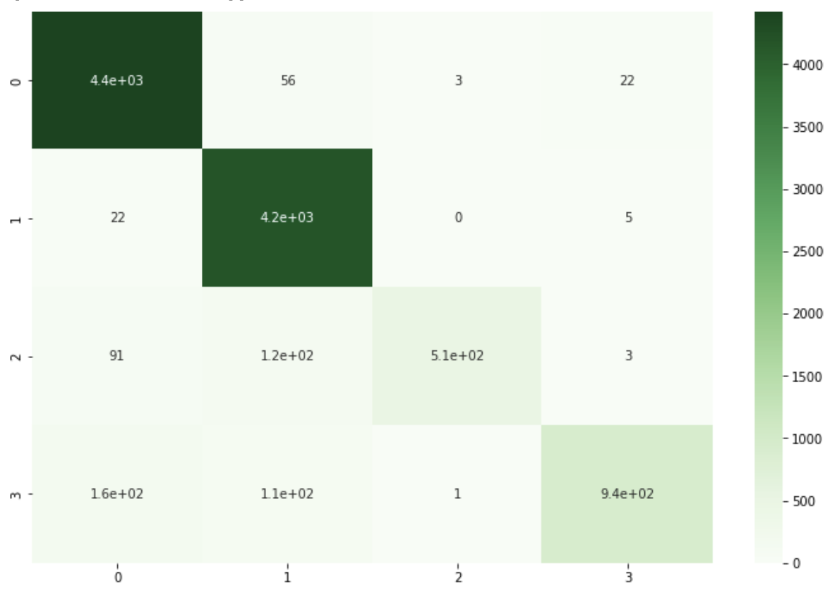
55. Confusion matrix

Create the confusion matrix of the logistic regression model from the problem 52 for both the training data and the test data.

from sklearn.metrics import confusion_matrix
import seaborn as sns
import matplotlib.pyplot as plt

# train data
train_cm = confusion_matrix(train['CATEGORY'], y_pred_train)
print(train_cm)
plt.figure(figsize=(12, 8))
sns.heatmap(train_cm, annot=True, cmap='Greens')
plt.show()

[[4421   56    3   22]
 [  22 4196    0    5]
 [  91  125  509    3]
 [ 162  111    1  945]]

confusion matrix 55

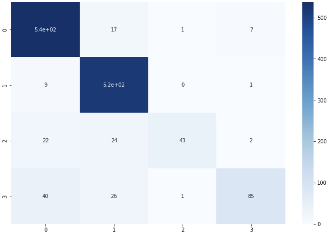
# test data
test_cm = confusion_matrix(test['CATEGORY'], y_pred_test)
print(test_cm)
plt.figure(figsize=(12, 8))
sns.heatmap(test_cm, annot=True, cmap='Blues')
plt.show()

[[538  17   1   7]
 [  9 518   0   1]
 [ 22  24  43   2]
 [ 40  26   1  85]]

confusion matrix 55

56. Precision, recall and F1 score

Compute the precision, recall and F1 score of the logistic regression model from the problem 52. First, compute these metrics for each category. Then summarize the score of each category using (1) micro-average and (2) macro-average.

from sklearn.metrics import precision_score, recall_score, f1_score
import numpy as np

# precision
precision = precision_score(test['CATEGORY'], y_pred_test, average=None, labels=model.classes_)
precision = np.append(precision, precision_score(test['CATEGORY'], y_pred_test, average='micro'))
precision = np.append(precision, precision_score(test['CATEGORY'], y_pred_test, average='macro'))

# recall
recall = recall_score(test['CATEGORY'], y_pred_test, average=None, labels=model.classes_)
recall = np.append(recall, recall_score(test['CATEGORY'], y_pred_test, average='micro'))
recall = np.append(recall, recall_score(test['CATEGORY'], y_pred_test, average='macro'))

# F1
f1 = f1_score(test['CATEGORY'], y_pred_test, average=None, labels=['b', 'e', 't', 'm'])
f1 = np.append(f1, f1_score(test['CATEGORY'], y_pred_test, average='micro'))
f1 = np.append(f1, f1_score(test['CATEGORY'], y_pred_test, average='macro'))

scores = pd.DataFrame({'precision': precision, 'recall': recall, 'F1': f1},
                    index=['b', 'e', 't', 'm', 'micro avg', 'macro avg'])

print(scores)

           precision    recall        f1
b           0.883415  0.955595  0.918089
e           0.885470  0.981061  0.930818
t           0.955556  0.472527  0.688259
m           0.894737  0.559211  0.632353
micro avg   0.887556  0.887556  0.887556
macro avg   0.904794  0.742098  0.792380

57. Feature weights

Use the logistic regression model from the problem 52. Check the feature weights and list the 10 most important features and 10 least important features.

features = x_train.columns.values
index = [i for i in range(1, 11)]
for c, coef in zip(model.classes_, model.coef_):
  print(f'category: {c}', '*' * 100)
  best_10 = pd.DataFrame(features[np.argsort(coef)[::-1][:10]], columns=['best 10'], index=index).T
  worst_10 = pd.DataFrame(features[np.argsort(coef)[:10]], columns=['worst 10'], index=index).T
  print(pd.concat([best_10, worst_10], axis=0))
  print('\n')

category: b ****************************************************************************************************
           1     2    3      4         5        6      7       8           9   \
best 10   fed  bank  ecb  china       oil  ukraine   euro  update      stocks
worst 10  and   the  her  ebola  facebook      she  video   study  kardashian

              10
best 10      buy
worst 10  google


category: e ****************************************************************************************************
                  1      2       3     4    5      6        7      8      9   \
best 10   kardashian  chris     kim   she  her  cyrus    miley   star   paul
worst 10      update     us  google  says  ceo  study  billion  china  could

                10
best 10      movie
worst 10  facebook


category: m ****************************************************************************************************
             1         2        3     4      5        6       7       8   \
best 10   ebola    cancer    study  drug    fda     mers  health   virus
worst 10     gm  facebook  climate   ceo  apple  twitter    deal  google

             9      10
best 10   could  heart
worst 10  sales    buy


category: t ****************************************************************************************************
              1         2      3        4          5         6        7   \
best 10   google  facebook  apple  climate  microsoft        gm  tmobile
worst 10     her        at   drug      fed        but  american   shares

               8           9       10
best 10   samsung  heartbleed   tesla
worst 10   cancer        bank  stocks

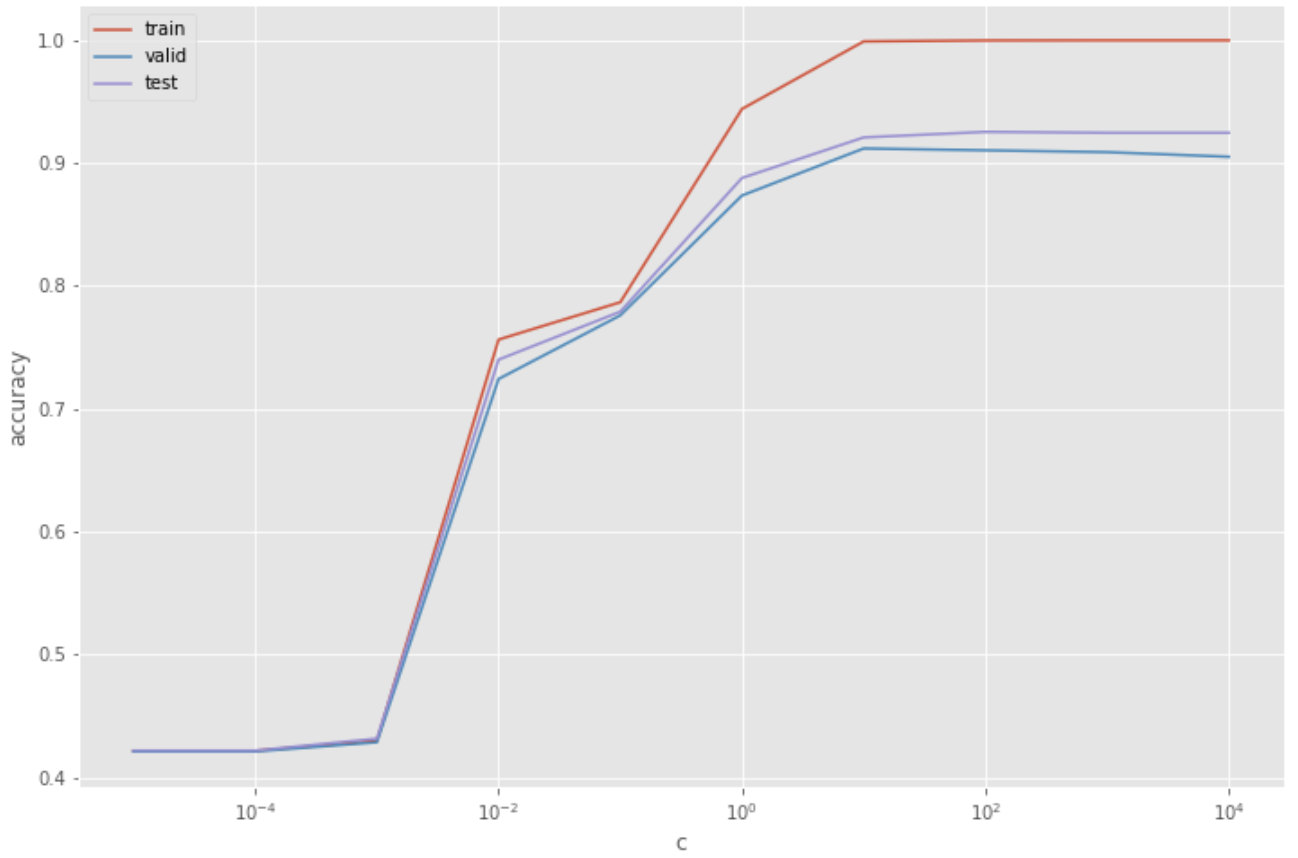
58. Regularization

When training a logistic regression model, one can control the degree of overfitting by manipulating the regularization parameters. Use different regularization parameters to train the model. Then, compute the accuracy score on the training data, validation data and test data. Summarize the results on the graph, where x-axis is the regularization parameter and y-axis is the accuracy score.

from tqdm import tqdm
import matplotlib.pyplot as plt

plt.style.use('ggplot')

c_list = np.logspace(-5, 4, 10, base=10)
# models = [LogisticRegression(C=C, random_state=42, max_iter=1000).fit(x_train, train['CATEGORY']) for C in tqdm(c_list)]

train_accs = [accuracy_score(model.predict(x_train), train['CATEGORY']) for model in models]
valid_accs = [accuracy_score(model.predict(x_valid), valid['CATEGORY']) for model in models]
test_accs = [accuracy_score(model.predict(x_test), test['CATEGORY']) for model in models]

plt.plot(c_list, train_accs, label = 'train')
plt.plot(c_list, valid_accs, label = 'valid')
plt.plot(c_list, test_accs, label = 'test')
plt.xscale('log')
plt.xlabel('c')
plt.ylabel('accuracy')
plt.legend()
plt.show()

59. Hyper-parameter tuning

Use different training algorithms and parameters to train the model for the news classification. Search for the training algorithms and parameters that achieves the best accuracy score on the validation data. Then compute its accuracy score on the test data.

!pip install optuna

import optuna

def objective(trial):
  model = LogisticRegression(random_state=42,
                             max_iter=10000,
                             penalty='elasticnet',
                             solver='saga',
                             l1_ratio=trial.suggest_uniform('l1_ratio', 0, 1),
                             C=trial.suggest_loguniform('C', 1e-4, 1e2))
  model.fit(x_train, train['CATEGORY'])
  valid_accuracy = accuracy_score(model.predict(x_valid), valid['CATEGORY'])

  return valid_accuracy

study = optuna.create_study(direction='maximize')
study.optimize(objective, n_trials=2, timeout=3600)

print('Best trial:')
trial = study.best_trial
print('  Value: {:.3f}'.format(trial.value))
print('  Params: ')
for key, value in trial.params.items():
  print('    {}: {}'.format(key, value))

>> Best trial:
>>   Value: 0.657
>>   Params:
>>     l1_ratio: 0.8173726339927334
>>     C: 0.08584685734174859

model = LogisticRegression(random_state=42,
                           max_iter=10000,
                           penalty='elasticnet',
                           solver='saga',
                           l1_ratio=trial.params['l1_ratio'],
                           C=trial.params['C'])
model.fit(x_train, train['CATEGORY'])

y_pred_train = model.predict(x_train)
y_pred_valid = model.predict(x_valid)
y_pred_test = model.predict(x_test)

train_accuracy = accuracy_score(train['CATEGORY'], y_pred_train)
valid_accuracy = accuracy_score(valid['CATEGORY'], y_pred_valid)
test_accuracy = accuracy_score(test['CATEGORY'], y_pred_test)

print(f'accuracy (train)：{train_accuracy:.3f}')
print(f'accuracy (valid)：{valid_accuracy:.3f}')
print(f'accuracy (test)：{test_accuracy:.3f}')

>> accuracy (train)：0.668
>> accuracy (valid)：0.657
>> accuracy (test)：0.653