What is Coefficient of Determination (R-squared)

The coefficient of determination, or R^2, is a statistical measure used in regression analysis to evaluate the goodness-of-fit of a model. It indicates the proportion of variation in the dependent variable that can be explained by the independent variable(s). R^2 ranges from 0 to 1, with 0 meaning that none of the variation in the dependent variable can be explained by the independent variable(s) and 1 meaning that all of the variation can be explained by them.

The formula for R^2 is:

where,

• y_i is the observed value of the dependent variable for the i^{th} data point.
• \hat{y_i} is the predicted value of the dependent variable for the i^{th} data point.
• \bar{y} is the mean value of the dependent variable.

R-squared and Goodness-of-Fit

Goodness-of-fit is a measure of how well a statistical model fits the observed data. A higher R^2 value indicates that the model fits the data better, as it accounts for a larger proportion of the variation in the dependent variable. However, it is important to remember that a high R^2 does not necessarily imply a causal relationship between the independent and dependent variables, and R^2 should not be the sole criterion for assessing model performance.

R-Squared and Correlation Coefficient

The correlation coefficient (r) is a measure of the strength and direction of the linear relationship between two variables. It ranges from -1 (perfect negative correlation) to 1 (perfect positive correlation), with 0 indicating no correlation. In simple linear regression, R^2 is equal to the square of the correlation coefficient, meaning that it shows the proportion of variation in the dependent variable that can be explained by the linear relationship with the independent variable. The formula for calculating R^2 in simple linear regression is:

Adjusted R-squared

Adjusted R^2 is a modification of R^2 that takes into account the number of independent variables and the sample size. It is particularly useful in multiple regression analysis, where the addition of independent variables can inflate the R^2 value, making the model appear to have a better fit than it actually does. The formula for adjusted R^2 is:

where n is the sample size and k is the number of independent variables.

Adjusted R^2 penalizes the model for adding independent variables that do not contribute significantly to the explained variance in the dependent variable, thus helping to prevent overfitting and aiding in model selection.

Calculating and Interpreting R-squared using Python

In this chapter, I will demonstrate how to calculate R-squared using Python and the California Housing dataset.

First, we will import the required libraries and load the California Housing dataset, a widely-used public dataset for regression analysis.

import numpy as np
import pandas as pd
import matplotlib.pyplot as plt
import seaborn as sns
from sklearn.linear_model import LinearRegression
from sklearn.metrics import r2_score
from sklearn.model_selection import train_test_split
from sklearn.datasets import fetch_california_housing

# Load the California Housing dataset
california = fetch_california_housing()
data = pd.DataFrame(california.data, columns=california.feature_names)
data['Price'] = california.target

Now, we will perform linear regression analysis using the LinearRegression class from the scikit-learn and calculate the R-squared value using the r2_score function. We will create two separate linear regression models using the good independent variable MedInc and the bad independent variable HouseAge. Then, we will calculate the R-squared values for both models.

# Good regression (MedInc vs. Price)
X_good = data[['MedInc']]
y_good = data['Price']

model_good = LinearRegression()
model_good.fit(X_good, y_good)

y_pred_good = model_good.predict(X_good)
r_squared_good = R-squared_score(y_good, y_pred_good)
print(f'R-squared (Good Regression - MedInc vs. Price): {r_squared_good:.2f}')

# Bad regression (HouseAge vs. Price)
X_bad = data[['HouseAge']]
y_bad = data['Price']

model_bad = LinearRegression()
model_bad.fit(X_bad, y_bad)

y_pred_bad = model_bad.predict(X_bad)
r_squared_bad = R-squared_score(y_bad, y_pred_bad)
print(f'R-squared (Bad Regression - HouseAge vs. Price): {r_squared_bad:.2f}')

R-squared (Good Regression - MedInc vs. Price): 0.47
R-squared (Bad Regression - HouseAge vs. Price): 0.01

As expected, the R-squared value for the good regression (MedInc vs. Price) is higher, indicating a better fit for the data. In contrast, the R-squared value for the bad regression (HouseAge vs. Price) is significantly lower, suggesting that the variable HouseAge does not provide a good fit for the data.

We will visualize the relationship between the dependent variable Price and a good independent variable MedInc, and a bad independent variable HouseAge.

# Good regression (MedInc vs. Price)
plt.figure(figsize=(10, 6))
sns.regplot(x='MedInc', y='Price', data=data, scatter_kws={'alpha': 0.3}, line_kws={'color': 'red'})
plt.title('Good Regression: MedInc vs. Price')
plt.xlabel('Median Income')
plt.ylabel('Price')
plt.show()

# Bad regression (HouseAge vs. Price)
plt.figure(figsize=(10, 6))
sns.regplot(x='HouseAge', y='Price', data=data, scatter_kws={'alpha': 0.3}, line_kws={'color': 'red'})
plt.title('Bad Regression: HouseAge vs. Price')
plt.xlabel('House Age')
plt.ylabel('Price')
plt.show()

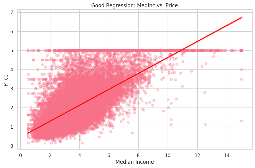
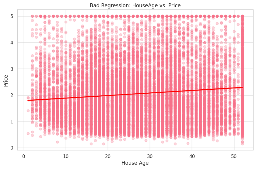
In the first plot, you can see a clear positive relationship between MedInc and Price. On the other hand, the second plot shows a weak relationship between HouseAge and Price.