2022-03-29

Correlation Coefficient

What is Correlation Coefficient

The correlation coefficient is a numerical measure that quantifies the strength and direction of the linear relationship between two continuous variables. Its primary purpose is to assess how closely the two variables are related and provide insights into the nature of their association. This chapter delves deeper into the two most commonly used correlation coefficients: Pearson's correlation coefficient ( $r$ ) and Spearman's rank correlation coefficient ( $\rho$ ).

Pearson's Correlation Coefficient

Pearson's correlation coefficient ( $r$ ) is calculated using the following formula:

r = \frac{\sum*{i=1}^{n}(x_i - \bar{x})(y_i - \bar{y})}{\sqrt{\sum*{i=1}^{n}(x*i - \bar{x})^2 \sum*{i=1}^{n}(y_i - \bar{y})^2}}

where:

$n$ is the number of paired data points
$x_i$ and $y_i$ are the individual data points
$\bar{x}$ and $\bar{y}$ are the means of the $x$ and $y$ variables, respectively

Spearman's Rank Correlation Coefficient

Spearman's rank correlation coefficient ( $\rho$ ) is calculated using the following formula:

\rho = 1 - \frac{6 \sum\_{i=1}^{n} d_i^2}{n(n^2 - 1)}

where:

$n$ is the number of paired data points
$d_i$ is the difference between the ranks of corresponding $x_i$ and $y_i$ values

Interpretation of Correlation

The value of correlation coefficient ranges from -1 to 1. The strength and direction of the correlation can be interpreted as follows:

-1 ≤ r < -0.7: Strong negative correlation
-0.7 ≤ r < -0.3: Moderate negative correlation
-0.3 ≤ r < 0: Weak negative correlation
0: No correlation
0 < r ≤ 0.3: Weak positive correlation
0.3 < r ≤ 0.7: Moderate positive correlation
0.7 < r ≤ 1: Strong positive correlation

Relationship between Covariance and Correlation Coefficient

Covariance and correlation coefficient are both measures of the relationship between two variables. While covariance provides information about the direction of the relationship (positive or negative), it does not provide any information about the strength of the relationship. In contrast, the correlation coefficient not only shows the direction of the relationship but also indicates the strength of the relationship on a standardized scale of -1 to 1.

The relationship between covariance and the Pearson's correlation coefficient can be expressed as follows:

r = \frac{cov(x, y)}{s_x s_y}

where:

$r$ is the Pearson's correlation coefficient
$cov(x, y)$ is the covariance between $x$ and $y$
$s_x$ and $s_y$ are the standard deviations of $x$ and $y$ , respectively

In this equation, the Pearson's correlation coefficient is obtained by dividing the covariance by the product of the standard deviations of the two variables. This process standardizes the covariance so that the resulting correlation coefficient lies between -1 and 1, making it easier to interpret the strength of the relationship.

Limitations and Assumptions of Correlation Coefficient

Both Pearson's $r$ and Spearman's $\rho$ have certain limitations and assumptions that should be considered when interpreting their values:

Correlation coefficients only measure the strength of the linear relationship between two variables; they do not imply causation.
Outliers or extreme values can significantly impact the correlation coefficient, potentially leading to misleading results. It is essential to visualize the data using scatterplots to identify any outliers and assess the true nature of the relationship.
Pearson's $r$ assumes that both variables are measured on an interval or ratio scale and that the relationship between them is linear. If these assumptions are not met, the results may be inaccurate.
Spearman's $\rho$ is more robust to outliers and non-linear relationships but requires at least one of the variables to be measured on an ordinal scale or for the relationship to be monotonic.
The correlation coefficient may be sensitive to the sample size; smaller sample sizes can result in weaker correlations, even if a strong relationship exists. It is important to ensure that the sample size is sufficiently large to accurately represent the population.

Calculating Correlation Coefficient with Python

In this chapter, I will demonstrate how to calculate correlation coefficient using Python.

First, let's import the necessary libraries.

python

import pandas as pd
import numpy as np
import seaborn as sns
import matplotlib.pyplot as plt

For this example, let's create a sample dataset with three variables: x, y, and z. We will use pandas to create a DataFrame containing the data.

python

data = {
    'x': [1, 2, 3, 4, 5, 6, 7, 8, 9, 10],
    'y': [2, 4, 6, 8, 10, 12, 14, 16, 18, 20],
    'z': [10, 9, 8, 7, 6, 5, 4, 3, 2, 1]
}

df = pd.DataFrame(data)

We can use the corr() method available in pandas DataFrame to calculate the correlation matrix for our dataset. The Pearson's correlation coefficient is used by default when using the corr() method in pandas DataFrame.

correlation_matrix = df.corr()
print(correlation_matrix)

     x    y    z
x  1.0  1.0 -1.0
y  1.0  1.0 -1.0
z -1.0 -1.0  1.0

To make the correlation matrix more visually appealing, we will use the seaborn to create a heatmap.

python

plt.figure(figsize=(10, 7))
sns.set(font_scale=1.2)
sns.heatmap(correlation_matrix, annot=True, cmap='coolwarm', annot_kws={"size": 12})
plt.title("Correlation Matrix")
plt.show()

Correlation matrix

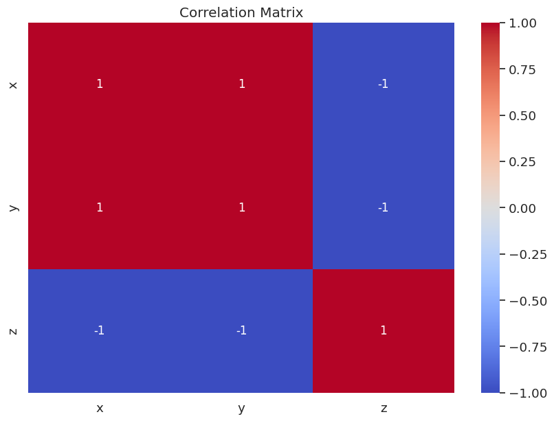
The resulting correlation matrix and heatmap will display the correlation coefficients for each pair of variables in the dataset.

The correlation coefficient between x and y is 1, indicating a strong positive correlation.
The correlation coefficient between x and z is -1, indicating a strong negative correlation.
The correlation coefficient between y and z is also -1, indicating a strong negative correlation.

By interpreting the correlation coefficients, we can gain insights into the relationships between the variables in our dataset. In this case, we can see that x and y have a strong positive linear relationship, while both x and z and y and z have strong negative linear relationships.

Visually Understanding Correlation

To demonstrate data with various correlation coefficients, we will generate three different datasets with varying degrees of correlation and create scatterplots for each dataset.

python

import numpy as np
import matplotlib.pyplot as plt

np.random.seed(42)

# Create dataset with a strong positive correlation
x1 = np.random.normal(50, 10, 100)
y1 = x1 * 1.2 + np.random.normal(0, 5, 100)

# Create dataset with a weak positive correlation
x2 = np.random.normal(50, 10, 100)
y2 = x2 * 0.2 + np.random.normal(0, 20, 100)

# Create dataset with no correlation
x3 = np.random.normal(50, 10, 100)
y3 = np.random.normal(50, 10, 100)

# Create scatterplots for each dataset
plt.figure(figsize=(18, 5))

plt.subplot(131)
plt.scatter(x1, y1)
plt.title("Strong Positive Correlation")
plt.xlabel("x1")
plt.ylabel("y1")

plt.subplot(132)
plt.scatter(x2, y2)
plt.title("Weak Positive Correlation")
plt.xlabel("x2")
plt.ylabel("y2")

plt.subplot(133)
plt.scatter(x3, y3)
plt.title("No Correlation")
plt.xlabel("x3")
plt.ylabel("y3")

plt.show()

Correlation

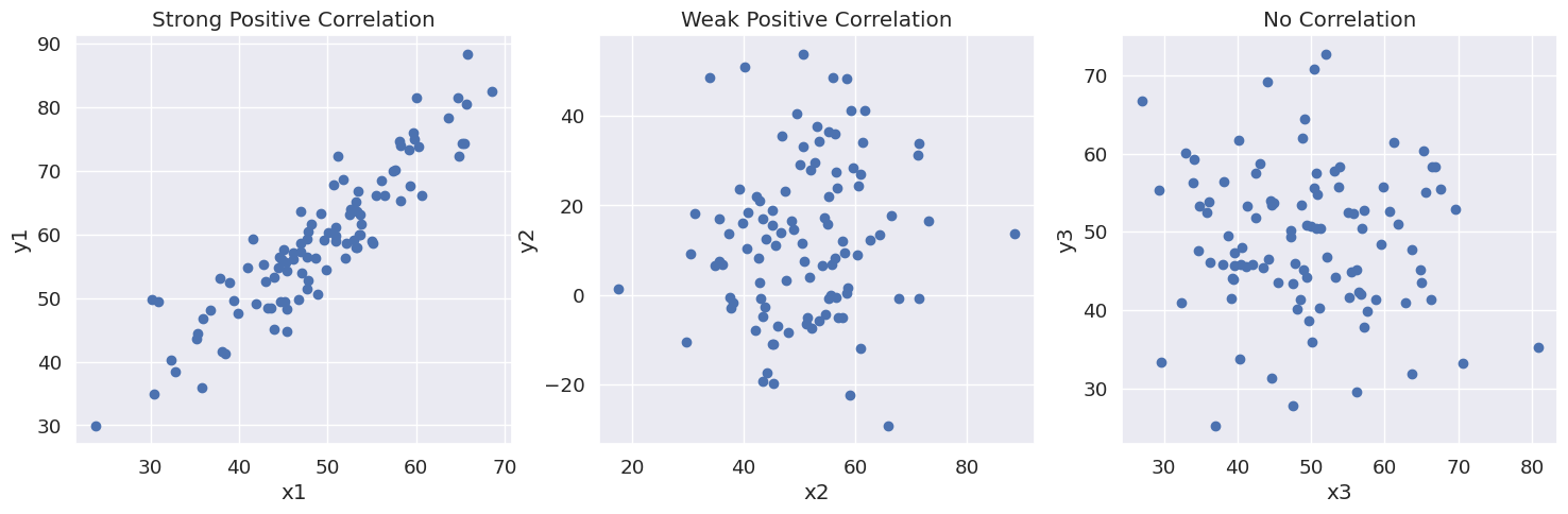
The code above generates three different datasets:

Strong positive correlation: In this dataset, x1 and y1 have a strong positive linear relationship, which is evident in the scatterplot as the points are closely clustered around a line with a positive slope.
Weak positive correlation: In this dataset, x2 and y2 have a weak positive linear relationship. The scatterplot shows that the points are dispersed around a line with a positive slope, but the dispersion is much greater than in the strong positive correlation case.
No correlation: In this dataset, x3 and y3 have no linear relationship. The scatterplot shows that the points are randomly distributed and do not follow any discernible pattern.