2022-10-01

Clustering

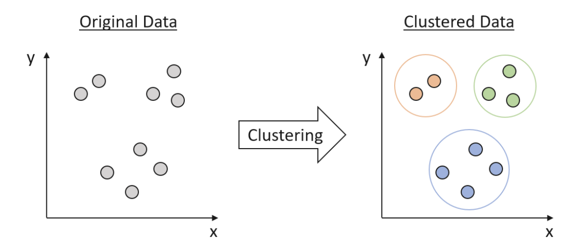
What is Clustering

Clustering is a fundamental technique in data science that helps uncover hidden patterns and structures in data. It is a form of unsupervised learning, which means that the algorithm attempts to identify the underlying structure of the data without any prior knowledge of its labels or categories. Clustering groups similar data points together based on their features, creating clusters that exhibit some degree of homogeneity. These clusters can then be used to understand the underlying relationships in the data and derive valuable insights.

Clustering basics and a demonstration in clustering infrastructure pathways

Distance Metrics

A fundamental concept in clustering is the measure of similarity or dissimilarity between data points. Distance metrics quantify the difference between data points, with smaller distances indicating greater similarity. Some of the commonly used distance metrics include:

Euclidean Distance
The most widely used distance metric, it calculates the straight-line distance between two points in Euclidean space.
Manhattan Distance
Also known as the L1 distance, it calculates the sum of the absolute differences between the coordinates of two points.
Cosine Similarity
Measures the cosine of the angle between two vectors, indicating their similarity. It is particularly useful when dealing with high-dimensional data or text data represented as term frequency vectors.
Mahalanobis Distance
Takes into account the correlations between features and is scale-invariant, making it useful when dealing with correlated or non-homogeneous data.
Jaccard Similarity
Measures the similarity between two sets by dividing the size of their intersection by the size of their union. It is often used for binary or categorical data.

Cluster Validity and Evaluation

Evaluating the quality of clustering results is crucial in determining the effectiveness of the chosen algorithm and its parameters. Cluster validity indices provide quantitative measures to assess the quality of clustering results. These indices can be divided into three categories:

Internal indices
Evaluate the clustering results based on the intrinsic properties of the data, such as within-cluster and between-cluster distances. Examples include the Silhouette index, the Davies-Bouldin index, and the Calinski-Harabasz index.
External indices
Compare the clustering results with a known ground truth, which is typically obtained from labeled data. Examples include the adjusted Rand index, the Fowlkes-Mallows index, and the Jaccard index.
Relative indices
Compare the performance of different clustering algorithms or parameter settings on the same dataset. Examples include the Gap statistic, the C-index, and the Dunn index.

Clustering Algorithms

K-means Clustering

K-means is a popular partition-based clustering algorithm that aims to minimize the within-cluster sum of squared distances. The algorithm iteratively assigns data points to one of the K predefined clusters based on their proximity to the cluster centroids, which represent the mean of all data points within a cluster. The main steps of the K-means algorithm are:

Initialize K cluster centroids randomly.
Assign each data point to the nearest centroid.
Update the centroids by computing the mean of all data points in each cluster.
Repeat steps 2 and 3 until convergence (i.e., centroids no longer change) or a predefined number of iterations is reached.

K-means is simple, fast, and scalable, making it suitable for large datasets and real-time applications. It works well when the data exhibits a clear partition structure with isotropic and convex-shaped clusters. However, K-means has several limitations:

It requires the user to specify the number of clusters (K) beforehand, which may not be known in advance.
The algorithm is sensitive to the initial placement of centroids and may converge to local minima. To mitigate this issue, multiple runs with different initializations can be performed, and the best solution can be selected based on the within-cluster sum of squared distances.
K-means is sensitive to outliers and noise, which can significantly impact the cluster centroids.
It assumes that all clusters have similar sizes, shapes, and densities, which may not hold true for real-world data.

Hierarchical Clustering

Hierarchical clustering algorithms build a tree-like structure (dendrogram) to represent the nested relationships between data points.

Dendrogram
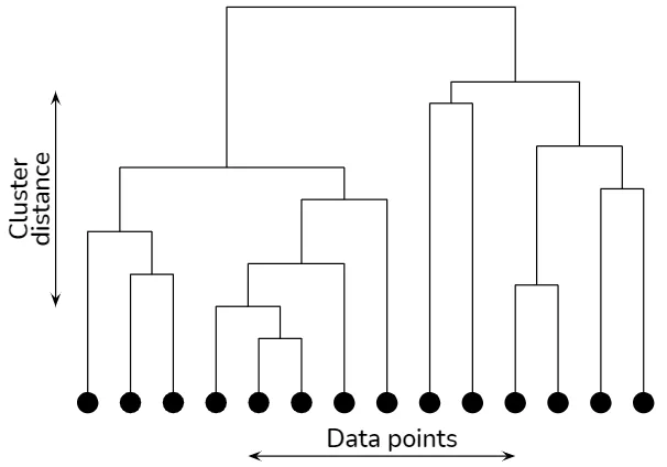
Hierarchical clustering explained

There are two main types of hierarchical clustering:

Agglomerative (bottom-up)
Starts with each data point as a separate cluster and iteratively merges the closest pair of clusters until a single cluster is obtained.
Divisive (top-down)
Starts with a single cluster containing all data points and recursively splits the cluster into smaller clusters based on some criterion.

The choice of the distance metric and linkage criterion, which determines how to compute the distance between clusters, significantly impacts the resulting dendrogram. Common linkage criteria include single-linkage, complete-linkage, average-linkage, and Ward's method.

DBSCAN (Density-Based Spatial Clustering of Applications with Noise)

DBSCAN is a density-based clustering algorithm that groups data points based on their proximity and density. The algorithm defines a cluster as a dense region of data points separated by areas of lower point density. DBSCAN requires two parameters: the neighborhood radius (eps) and the minimum number of points required to form a dense region (minPts). The main steps of the DBSCAN algorithm are:

For each data point, determine its neighbors within the eps radius.
If a data point has at least minPts neighbors, mark it as a core point; otherwise, mark it as a noise point.
For each core point not yet assigned to a cluster, create a new cluster and recursively add all directly and indirectly reachable core points to the cluster.
Assign noise points to the nearest cluster if they are within the eps radius of a core point; otherwise, leave them unassigned.

DBSCAN is robust against noise, as it can identify and separate noise points from clusters. It can also detect clusters with arbitrary shapes and varying densities, unlike K-means and hierarchical clustering. However, DBSCAN requires the user to define the eps and minPts parameters, which can be challenging. A common approach to selecting these parameters is using the k-distance graph, where the distance to the k-th nearest neighbor is plotted for each data point in ascending order.

Gaussian Mixture Models

A Gaussian Mixture Model (GMM) is a generative probabilistic model that represents a dataset as a mixture of several Gaussian distributions. The Expectation-Maximization (EM) algorithm is used to estimate the parameters of the Gaussian distributions and the mixing proportions. The main steps of the EM algorithm are:

Initialize the Gaussian distribution parameters and the mixing proportions.
E-step: Calculate the posterior probabilities of each data point belonging to each Gaussian distribution, given the current parameter estimates.
M-step: Update the Gaussian distribution parameters and the mixing proportions based on the posterior probabilities.
Repeat steps 2 and 3 until convergence or a predefined number of iterations is reached.

GMMs can model complex data distributions and automatically estimate the covariance structure of the clusters. However, the user needs to specify the number of Gaussian distributions (components) beforehand. Model selection techniques, such as the AIC and the Bayesian Information Criterion (BIC), can be used to choose the optimal number of components.

Spectral Clustering

Spectral clustering is a graph-based clustering technique that leverages the spectral properties of the graph Laplacian matrix to identify clusters in the data. The algorithm starts by constructing a similarity graph, where each data point is a node, and the edge weights represent the pairwise similarities between data points. The graph Laplacian matrix is then computed, and its eigenvectors are used to perform dimensionality reduction and clustering.

Spectral clustering is particularly effective in detecting non-convex clusters and handling data with complex structures. However, it can be computationally expensive for large datasets due to the eigendecomposition of the Laplacian matrix. Various approximation techniques, such as the Nyström method and randomized algorithms, can be employed to improve the scalability of spectral clustering.