68-95-99.7 Rule in Normal Distribution

The normal distribution is a fundamental concept in the field of statistics and probability. It has numerous applications across various disciplines, from social sciences to natural sciences and engineering. One of the essential characteristics of the normal distribution is the 68-95-99.7 rule, also known as the Empirical Rule.

Understanding 68-95-99.7 Rule

The Empirical Rule is based on the properties of the normal distribution curve, which is symmetric and bell-shaped. In a normal distribution, the mean, median, and mode coincide, and the curve is entirely determined by its mean (\mu) and standard deviation (\sigma). The standard deviation is a measure of dispersion or spread in a dataset, indicating how closely the data points cluster around the mean.

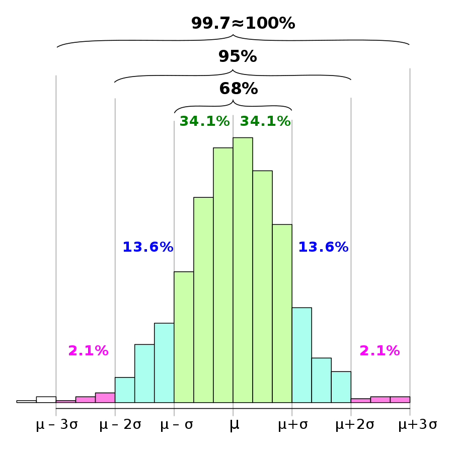
The 68-95-99.7 rule states that, in a normal distribution:

• Approximately 68% of the data falls within one standard deviation (\mu\pm\sigma) of the mean.
• About 95% of the data lies within two standard deviations (\mu\pm2\sigma) of the mean.
• Roughly 99.7% of the data falls within three standard deviations (\mu\pm3\sigma) of the mean.

These percentages arise from the mathematical properties of the normal distribution and serve as a practical tool for analyzing data that follows this distribution.

68–95–99.7 rule

Visualizing 68-95-99.7 Rule

In this chapter, I will demonstrate how to visualize the 68-95-99.7 rule using Python. We will generate a normally distributed dataset and create a plot that highlights the Empirical Rule's percentages.

Here is the code:

import numpy as np
import matplotlib.pyplot as plt
import seaborn as sns
from scipy.stats import norm

# Set the Seaborn style
sns.set(style="whitegrid")

# Parameters for the normal distribution
mean = 0
std_dev = 1
sample_size = 1000

# Generate the dataset
data = np.random.normal(mean, std_dev, sample_size)

plt.figure(figsize=(10, 6))

# Calculate the x values within each standard deviation range
x = np.linspace(mean - 3.5 * std_dev, mean + 3.5 * std_dev, 1000)
x1 = np.linspace(mean - std_dev, mean + std_dev, 1000)
x2 = np.linspace(mean - 2 * std_dev, mean + 2 * std_dev, 1000)
x3 = np.linspace(mean - 3 * std_dev, mean + 3 * std_dev, 1000)

# Get the corresponding y values for the normal distribution
y = norm.pdf(x, mean, std_dev)

# Plot the areas under the curve
plt.fill_between(x3, 0, norm.pdf(x3, mean, std_dev), color='darkblue', alpha=0.3, label='99.7%')
plt.fill_between(x2, 0, norm.pdf(x2, mean, std_dev), color='mediumblue', alpha=0.4, label='95%')
plt.fill_between(x1, 0, norm.pdf(x1, mean, std_dev), color='lightblue', alpha=0.5, label='68%')

# Customize the appearance
plt.plot(x, y, color='darkblue', linewidth=2)
plt.title('Visualizing the 68-95-99.7 Rule in Normal Distribution', fontsize=16)
plt.xlabel('Standard Deviations from the Mean', fontsize=14)
plt.ylabel('Density', fontsize=14)
plt.legend(title='Percentage', fontsize=12, title_fontsize=12)

# Display the plot
plt.show()

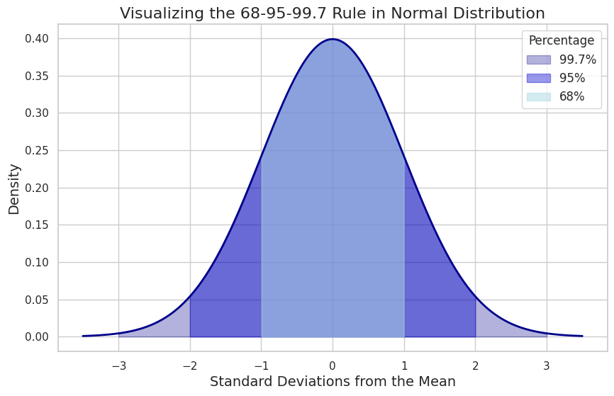
This code will generate a plot that illustrates the 68-95-99.7 rule in the context of a normal distribution. The shaded areas represent the percentages of data within one, two, and three standard deviations from the mean, as specified by the Empirical Rule.