Introduction

XGBoost is an open-source software library that provides an efficient and user-friendly implementation of the gradient boosting algorithm. Designed to be scalable and high-performing, XGBoost has quickly gained popularity among data scientists and machine learning practitioners for its ability to deliver state-of-the-art results on a wide range of machine learning problems.

This article will walk you through the process of installing and setting up XGBoost, introducing you to its basic workflow and API, as well as exploring feature importance in XGBoost models.

Installation and Setup

Before installing XGBoost, make sure you have the following software installed on your system:

• Python 3.6 or later
• NumPy
• SciPy
• scikit-learn

To install XGBoost, simply run the following command in your terminal or command prompt:

$ pip install xgboost

Basic XGBoost Workflow

In this chapter, I will walk through a basic XGBoost workflow, which includes loading a public dataset, preprocessing the data, creating a train and test split, defining and training the model, and evaluating its performance.

Loading a Public Dataset

For our XGBoost implementation, we will use the famous Iris dataset, which is available in the scikit-learn. This dataset contains 150 samples of iris flowers, each with four features (sepal length, sepal width, petal length, and petal width) and a corresponding class label (setosa, versicolor, or virginica).

First, let's import the necessary libraries and load the dataset:

import numpy as np
import pandas as pd
from sklearn import datasets

iris = datasets.load_iris()
X = iris.data
y = iris.target

Preprocessing the Data

Before we proceed with the XGBoost model, it's essential to preprocess the data. In this case, we will only perform label encoding for the target variable (class labels) to convert them into integer values.

from sklearn.preprocessing import LabelEncoder

encoder = LabelEncoder()
y_encoded = encoder.fit_transform(y)

Creating a Train and Test Split

To evaluate the performance of our XGBoost model, we need to divide the dataset into training and testing sets. We will use 80% of the data for training and the remaining 20% for testing.

from sklearn.model_selection import train_test_split

X_train, X_test, y_train, y_test = train_test_split(X, y_encoded, test_size=0.2, random_state=42)

Defining and Training the Model

Now that our data is ready, we can define our XGBoost model. Since this is a classification problem, we will use the XGBClassifier class.

from xgboost import XGBClassifier

model = XGBClassifier()
model.fit(X_train, y_train)

Model Evaluation and Prediction

With our XGBoost model trained, we can now evaluate its performance on the test dataset and make predictions. We will use accuracy as the evaluation metric.

from sklearn.metrics import accuracy_score

y_pred = model.predict(X_test)
accuracy = accuracy_score(y_test, y_pred)

print(f"Model accuracy: {accuracy:.2f}")

Model accuracy: 1.00

Exploring XGBoost's API

In this chapter, I will dive deeper into XGBoost's API and explore some of its powerful features, such as the XGBClassifier and XGBRegressor classes, the DMatrix data structure, cross-validation, early stopping, and custom evaluation metrics.

XGBClassifier and XGBRegressor Classes

XGBoost provides two main classes for implementing gradient boosting models: XGBClassifier for classification problems and XGBRegressor for regression problems. Both classes offer several hyperparameters to fine-tune the model's performance, such as:

• n_estimators: The number of boosting rounds (default: 100).
• learning_rate: The step size shrinkage used in the update to prevent overfitting (default: 0.3).
• max_depth: The maximum depth of a tree (default: 6).
• subsample: The fraction of samples to be used for fitting the individual base learners (default: 1).
• colsample_bytree: The fraction of features to choose for each boosting round (default: 1).

The DMatrix Data Structure

XGBoost uses a custom data structure called DMatrix to store datasets internally. The DMatrix format is optimized for both memory efficiency and training speed. To create a DMatrix, you can use the following code:

import xgboost as xgb

dtrain = xgb.DMatrix(X_train, label=y_train)
dtest = xgb.DMatrix(X_test, label=y_test)

When using the DMatrix format, you can use XGBoost's native API for training and predicting:

params = {'objective': 'multi:softmax', 'num_class': 3}
model = xgb.train(params, dtrain, num_boost_round=100)
y_pred = model.predict(dtest)

Cross-validation with XGBoost

XGBoost provides a built-in function for performing k-fold cross-validation, which can help you fine-tune your model's hyperparameters and assess its performance. To perform cross-validation, use the cv function:

cv_results = xgb.cv(params, dtrain, num_boost_round=100, nfold=5, metrics='merror', early_stopping_rounds=10)

Here, nfold specifies the number of folds for cross-validation, metrics is the evaluation metric used, and early_stopping_rounds stops training if the performance doesn't improve for the specified number of rounds.

Early Stopping and Custom Evaluation Metrics

Early stopping is a useful technique to prevent overfitting by stopping the training process if the model's performance on a validation set doesn't improve for a specified number of rounds. You can use early stopping in XGBoost by providing a validation set and specifying the early_stopping_rounds parameter during training:

model = xgb.train(params, dtrain, num_boost_round=100, evals=[(dtest, 'validation')], early_stopping_rounds=10)

XGBoost also allows you to define custom evaluation metrics. To implement a custom metric, you need to create a Python function that takes two arguments: the predicted values and a DMatrix object containing the true labels. The function should return a tuple containing the metric's name and its value. For example, you can create a custom accuracy metric as follows:

def accuracy_metric(preds, dmatrix):
    labels = dmatrix.get_label()
    return 'accuracy', accuracy_score(labels, preds)

model = xgb.train(params, dtrain, num_boost_round=100, evals=[(dtest, 'validation')], feval=accuracy_metric, early_stopping_rounds=10)

This code snippet demonstrates how to use the custom accuracy_metric during training by passing it as the feval parameter. The model will now be evaluated using the custom accuracy metric, and early stopping will be applied based on its performance.

Feature Importance in XGBoost

Feature importance is a technique used to identify and rank the most important features in a dataset based on their contribution to the model's predictions. Understanding feature importance can help you gain insights into the relationships between features and the target variable, as well as improve model interpretability. In this chapter, I will explore different types of feature importance in XGBoost and learn how to plot and interpret the results.

Feature Importance Types

XGBoost provides several importance types that can be used to rank features based on different criteria. The most common importance types are:

• weight: The number of times a feature appears in the trees across all boosting rounds.
• gain: The average gain (improvement in the splitting criterion) of a feature when it is used in the trees.
• cover: The average coverage of a feature when it is used in the trees.

Plotting Feature Importance

For example, to plot the gain-based feature importance for the Iris dataset, you can use the following code:

import seaborn as sns
import xgboost as xgb

# Set Seaborn's plotting style and color palette
sns.set_style("whitegrid")
sns.set_palette("husl")

# Obtain feature importance values
importance_df = pd.DataFrame(model.get_booster().get_score(importance_type='gain').items(),
                             columns=['Feature', 'Importance'])

# Sort dataframe by importance values
importance_df = importance_df.sort_values(by='Importance', ascending=False)

# Plot the feature importance using Seaborn's barplot
plt.figure(figsize=(10, 6))
sns.barplot(x='Importance', y='Feature', data=importance_df)
plt.title('Gain-based Feature Importance for Iris Dataset', fontsize=18)
plt.xlabel('Importance (F score)', fontsize=14)
plt.ylabel('Feature', fontsize=14)
plt.show()

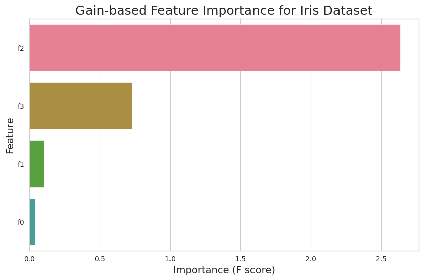
This code snippet will generate a bar chart showing the gain-based feature importance for each feature in the Iris dataset. You can replace 'gain' with 'weight' or 'cover' to plot the respective importance types.

Interpreting the Results

The feature importance plot provides valuable insights into the relationships between features and the target variable. Features with higher importance values have a greater impact on the model's predictions, while features with lower importance values contribute less.

References

https://xgboost.readthedocs.io/en/stable/