2023-02-03

Principal Component Analysis (PCA)

What is PCA

Principal Component Analysis (PCA) is a widely used technique in the realm of data science, particularly for dimensionality reduction, data visualization, and noise reduction. This powerful method enables researchers and practitioners to analyze and uncover the hidden patterns within large and complex datasets, which can lead to valuable insights and improved decision-making.

The Essence of PCA

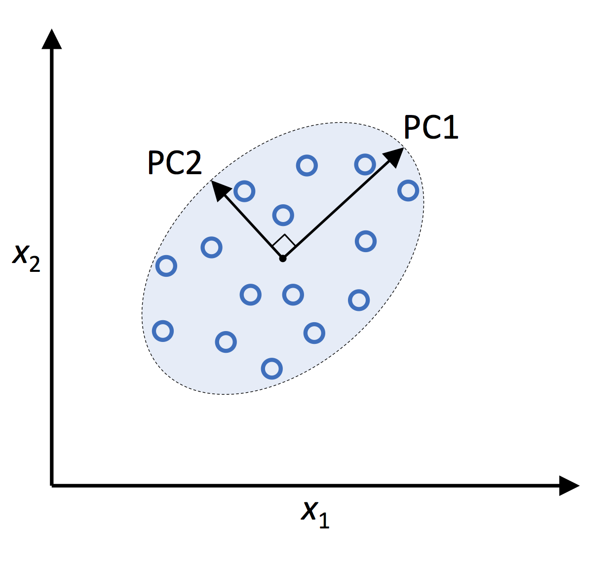
The primary goal of PCA is to reduce the dimensionality of a dataset while retaining as much information as possible. This is achieved by transforming the original features into a new set of orthogonal features, called principal components (PCs), which are linear combinations of the original variables. The PCs are ranked in order of their variance, with the first principal component accounting for the most variance in the data, followed by the second, and so on. By retaining only a subset of PCs, one can effectively reduce the dimensionality of the dataset and simplify analysis without losing significant information.

Principal Components
Python Machine Learning (2nd Ed.) Code Repository

Mathematics of PCA

In this chapter, I delve into the mathematical foundations of PCA. To understand the underlying concepts and techniques, a basic knowledge of linear algebra and statistics is essential.

Linear Algebra and Eigenvalues

PCA relies on linear algebra concepts, specifically eigenvalues and eigenvectors. Given a square matrix $A$ , an eigenvector $v$ is a non-zero vector that satisfies the following equation:

Av = \lambda v

where $\lambda$ is the eigenvalue associated with the eigenvector $v$ . In the context of PCA, eigenvalues and eigenvectors play a crucial role in transforming the original dataset into a new set of uncorrelated variables (principal components).

Covariance Matrix

The covariance matrix is a key element in PCA, as it captures the relationships between the original variables in the dataset. For a dataset $X$ with $n$ samples and $p$ features, the covariance matrix $C$ is a $p$ x $p$ symmetric matrix, with each element $c_ij$ representing the covariance between feature $i$ and feature $j$ :

C_{ij} = \frac{1}{n-1} \sum_{k=1}^{n}(x_{ki} - \bar{x}i)(x{kj} - \bar{x}_j)

where $x_ki$ is the value of feature $i$ for sample $k$ , and $\bar{x}_j$ is the mean value of feature $i$ across all samples.

Eigendecomposition

Eigendecomposition is the process of decomposing a matrix into its eigenvalues and eigenvectors. In PCA, we perform eigendecomposition on the covariance matrix $C$ , which results in a set of eigenvalues and their corresponding eigenvectors. The eigenvectors corresponding to the largest eigenvalues represent the directions in which the data has the highest variance, and thus form the basis for the principal components.

Dimensionality Reduction

Once we have the eigenvalues and eigenvectors of the covariance matrix, we can reduce the dimensionality of the dataset by selecting the top $k$ eigenvectors associated with the k largest eigenvalues. These eigenvectors, also known as the principal components, are then used to transform the original dataset $X$ into a new dataset $Y$ with reduced dimensions:

Y = XW_k

where $W_k$ is a $p$ x $k$ matrix containing the top $k$ eigenvectors as its columns. The new dataset $Y$ now has $k$ features, which are linear combinations of the original $p$ features and represent the directions of maximum variance in the data. By retaining only a subset of principal components, we can effectively reduce the dimensionality of the dataset while preserving most of the original information.

PCA in Practice

In this chapter, I will walk through a step-by-step guide on performing PCA using a publicly available dataset - the famous Iris dataset. This dataset contains 150 samples of iris flowers, with four features: sepal length, sepal width, petal length, and petal width. The objective is to reduce the dimensionality of the dataset while preserving its inherent structure.

Data Preprocessing

Before performing PCA, it is essential to preprocess the data. The main preprocessing step is standardization. Standardization scales the features to have a mean of 0 and a standard deviation of 1. This step is necessary for PCA to work effectively.

Here's how to preprocess the Iris dataset using Python and the scikit-learn library:

python

import numpy as np
import pandas as pd
from sklearn import datasets
from sklearn.preprocessing import StandardScaler

# Load the Iris dataset
iris = datasets.load_iris()
X = iris.data

# Standardize the data
scaler = StandardScaler()
X_scaled = scaler.fit_transform(X)

Implementing PCA

Now that the data is preprocessed, we can perform PCA using the scikit-learn library. Here's the code to reduce the Iris dataset to two dimensions:

python

from sklearn.decomposition import PCA

# Perform PCA with 2 components
pca = PCA(n_components=2)
X_pca = pca.fit_transform(X_scaled)

Interpretation of PCA Results

The output of PCA is a new dataset (X_pca) with reduced dimensions. In our example, we've reduced the Iris dataset from four dimensions to two. To understand the importance of each principal component, we can examine the explained variance ratio, which indicates the proportion of the total variance in the data explained by each component:

python

explained_variance_ratio = pca.explained_variance_ratio_
print(explained_variance_ratio)

The output might be something like:

array([0.72962445, 0.22850762])

This indicates that the first principal component explains approximately 72.96% of the total variance in the data, while the second principal component explains about 22.85%. Together, these two components account for roughly 95.81% of the total variance.

Visualizing PCA Components

Finally, we can visualize the PCA-transformed data in a scatter plot. This will allow us to observe any patterns or clusters in the reduced-dimensionality dataset. Here's the code to create a scatter plot of the two principal components using the matplotlib:

python

import matplotlib.pyplot as plt

# Plot the PCA-transformed data
plt.scatter(X_pca[:, 0], X_pca[:, 1], c=iris.target, cmap='viridis', edgecolor='k', s=75)
plt.xlabel('First Principal Component')
plt.ylabel('Second Principal Component')
plt.title('PCA with 2 Components on Iris Dataset')
plt.show()

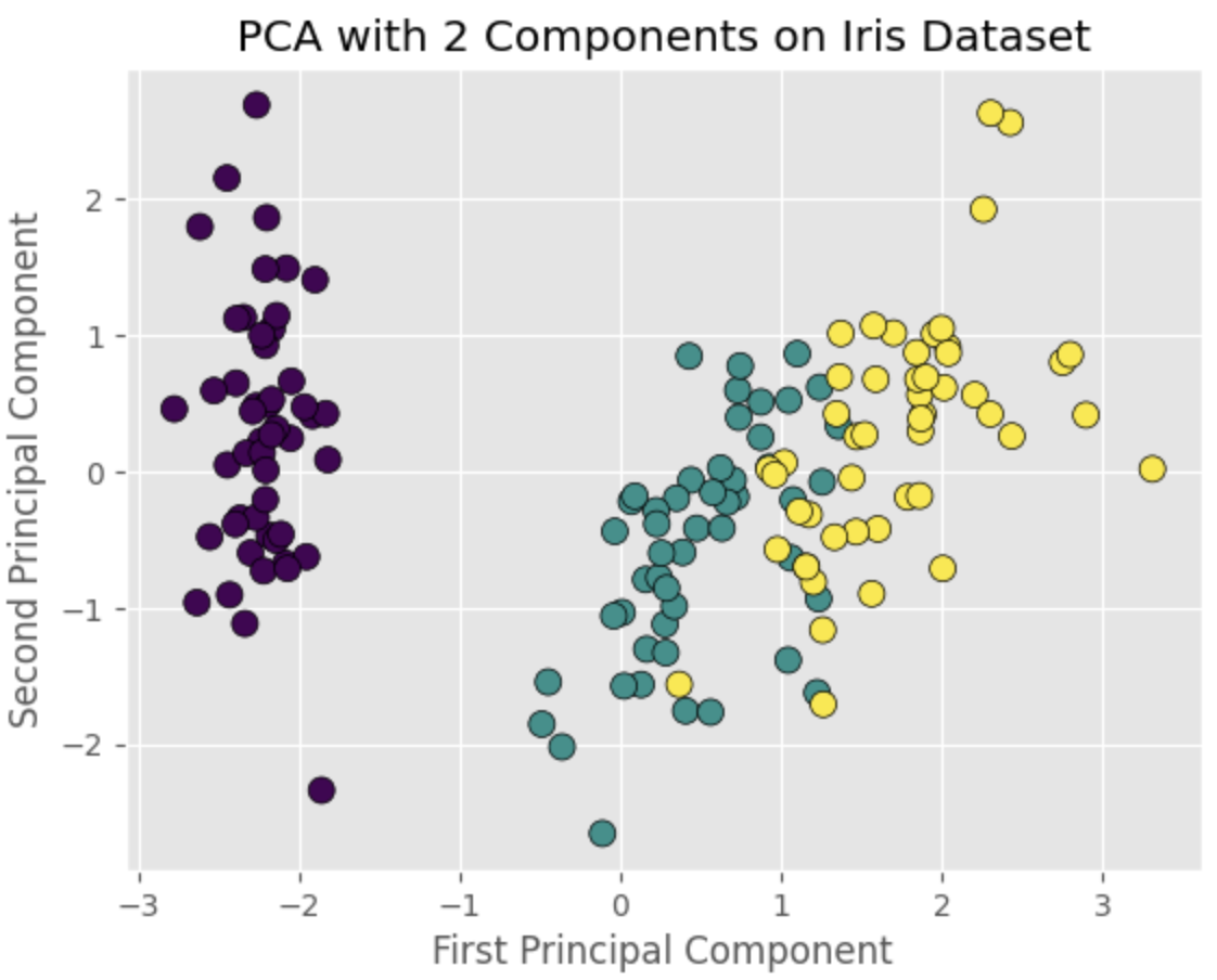
PCA with 2 Components on Iris Dataset

The scatter plot will show distinct clusters corresponding to the three iris species, demonstrating that PCA can effectively reduce the dimensionality of the data while preserving its structure.

Principal Component Loadings

Principal component loadings, also known as component loadings or eigenvector loadings, are the coefficients that indicate how each original feature contributes to a particular principal component. Analyzing the loadings can help us understand the relationships between the original features and the principal components, as well as the underlying structure of the data.

Here's how to obtain the principal component loadings for the Iris dataset using the PCA model we implemented earlier:

python

loadings = pca.components_
print(loadings)

The output might be something like:

array([[ 0.52106591, -0.26934744,  0.5804131 ,  0.56485654],
       [ 0.37741762,  0.92329566,  0.02449161,  0.06694199]])

This array represents the loadings for the two principal components, with each row corresponding to a principal component and each column corresponding to an original feature. The higher the absolute value of a loading, the stronger the contribution of the corresponding original feature to the principal component.

For instance, in the first principal component, petal length (0.580) and petal width (0.565) have higher loadings compared to sepal length (0.521) and sepal width (-0.269). This suggests that the first principal component is largely driven by the variation in petal length and petal width.

To visualize the loadings, we can create a biplot, which is a scatter plot of the PCA-transformed data overlaid with vectors representing the loadings:

python

def biplot(X_pca, loadings, labels=None):
    plt.figure(figsize=(10, 7))
    plt.scatter(X_pca[:, 0], X_pca[:, 1], c=iris.target, cmap='viridis', edgecolor='k', s=75)

    if labels is None:
        labels = np.arange(loadings.shape[1])

    for i, label in enumerate(labels):
        plt.arrow(0, 0, loadings[0, i], loadings[1, i], color='r', alpha=0.8, lw=2)
        plt.text(loadings[0, i] * 1.15, loadings[1, i] * 1.15, label, color='r', ha='center', va='center', fontsize=12)

    plt.xlabel('First Principal Component')
    plt.ylabel('Second Principal Component')
    plt.title('PCA Biplot of Iris Dataset')
    plt.grid()
    plt.show()

feature_labels = iris.feature_names
biplot(X_pca, loadings, labels=feature_labels)

PCA Biplot of Iris Dataset

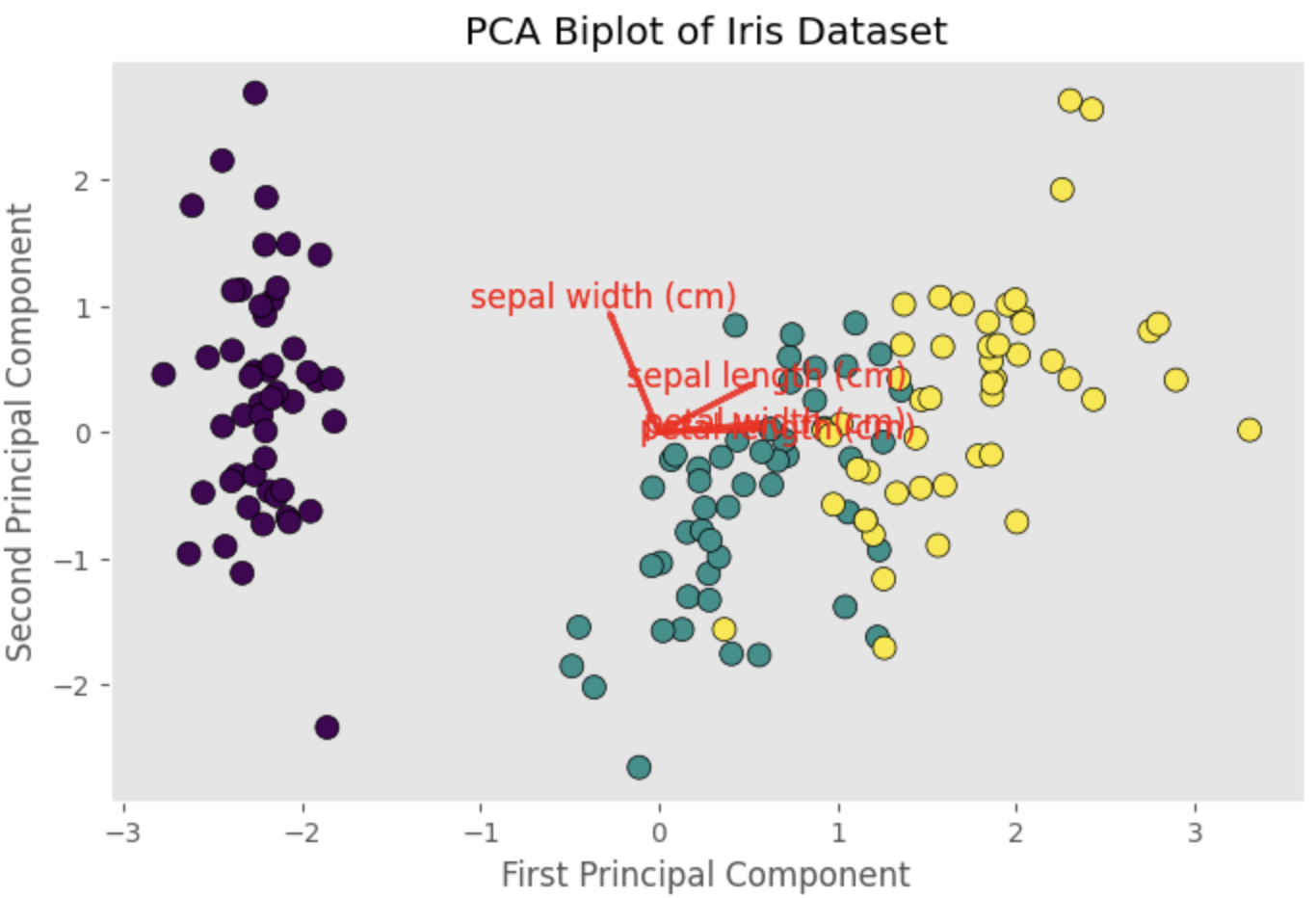
The biplot will display vectors representing the loadings for sepal length, sepal width, petal length, and petal width. The direction and length of each vector indicate the contribution of the corresponding feature to the principal components. By examining the biplot, we can gain insights into the relationships between the original features and the principal components, as well as the structure of the data.